Blind deconvolution #4: Blind deconvolution
Published on 31st of May, 2021.
In this final part on the deconvolution series, we will look at blind deconvolution. That is, we want to remove blur from images while having only partial knowledge about how the image was blurred. First of all we will develop a simple method to generate somewhat realistic forms of combined motion and gaussian blur. Then we will try a modification of the Richardson-Lucy deconvolution algorithm as a method for blind deconvolution – this doesn’t work very well, but does highlight a common issue with deconvolution algorithms. Then finally we will combine the image priors discussed in part 2 with Bayesian optimization to get a decent (but slow) method for blind deconvolution.
Realistic blur
What constitutes as ‘realistic’ blur obviously depends on context, but in the case of taking pictures with a hand-held camera or smartphone, it includes both motion blur and a form of lens blur. Generating lens blur is easy; we can just use a Gaussian blur. For motion blur we previously looked only at straight lines, but this isn’t very realistic. Natural motion is rarely just in a straight line, but is more erratic.
To model this we can take inspiration from physical processes such as Brownian motion: we can model motion blur as the path taken by a particle with an initial velocity, which is constantly perturbed during the motion. We want to add gaussian blur on top of that, which can simply be done by taking the image of such a path and convolving it with a gaussian point spread function. However, we should also take into account the speed of the particle; if we move a camera very fast then the camera spends less exposure time in any particular point. Therefore we should make the intensity of the blur inversely proportional to the speed at any point. The end result looks something like this:
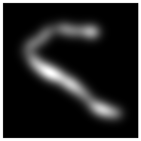
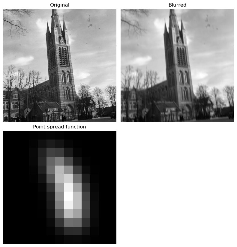
In practice we will consider this kind of blur at a much smaller resolution, for example of size 15x15. Below we show how such a kernel will affect for example the St. Vitus image.
Richardson-Lucy blind deconvolution
Recall that in the Richardson-Lucy algorithm we try to solve the deconvolution problem by using an iteration of form
This method is completely symmetric in and , so given an estimate of we can recover the kernel by the same method:
A simple idea for blind deconvolution is therefore to alternatingly estimate from and vice-versa. We can see the result of this procedure below:
The problem with this Richardson-Lucy-based algorithm is that the point spread function tends to converge to a (shifted) delta function. This is an inherit problem with many blind deconvolution algorithm, especially those based on finding a maximum a posteriori (MAP) estimate of both the kernel and image combined. For this particular algorithm it isn’t immediately obvious why it tends to do this, since the analysis of this algorithm is relatively complicated. Somehow the kernel update step tends to promote sparsity. This tends to happen irrespective of how we initialize the point spread function, or the relative number of steps spent estimating the PSF or the image.
There are heuristic ways to get around this, but overall it is difficult to make a technique like this work well. It also doesn’t use the wonderful things we learned about image priors in part 2. We need a method that can actively avoid converging to extreme points such as this delta function.
Parametrizing the point spread functions
In part 2 we discussed different image priors, of which the most promising prior is based on non-local self-similarity. This assigns to an image a score signifying how ‘natural’ this image is. We saw that it indeed gave higher scores for images that are appropriately sharpened. A simple idea is then to try different point spread functions, and use the one with the highest score. If we denote the result of applying deconvolution with kernel , then we want to solve the maximization problem:
If we naively try to maximize this function we run into the problem that the space of all kernels is quite large; a kernel obviously need parameters. Since computing the image prior is relatively expensive (as is the deconvolution), exploring this large space is not feasible. Moreover, the function is relatively noisy, and has the problem that it can give large scores to oversharpened images.
We therefore need a way to describe the point spread functions using only a few parameters. Moreover, this description should actively avoid points that are not interesting, such as a delta function or a point spread function that would result in heavy oversharpening of the image.
There are many ways to describe a point spread function using only a couple parameters. One way that I propose is by writing it as a sum of a small number of Gaussian point spread functions. However instead of having the centered symmetric Gaussians we have considered so far, we will allow an arbitrary mean and covariance matrix. This changes respectively the center and the shape of the point spread function. That is, it depends on the parameters and a 2x2 (symmetric, positive definite) matrix . Then the point spread function is given by
To be precise, we can describe the covariance matrix using three parameters and using the decomposition
We then use an additional parameter to combine different kernels of this type. By taking
This gives a total of 6 parameters per mixture component, but for the first component we can set the mean to and use a magnitude of 1, reducing to 3 parameters. For now we will try to use a mix just use two mixture components , and focus our attention on how to optimize this.
Bayesian optimization for blind deconvolution
We now know how to parameterize the point spread functions, and what function we want to optimize (the image prior). Next is deciding how to optimize this. In this case we have a complicated, noisy function that is expensive to compute, and with no easy way to compute its derivatives. In situations like these Bayesian optimization or other methods of ‘black-box’ optimization make the most sense.
How this works is that we sample our function in several points , where is our parameter searchspace. Based on these samples, we build a surrogate model for the function . We can then optimize the surrogate model to obtain a new point . We then compute , and update the surrogate model with this new information. This is then repeated a number of times, or until convergence. So long as the surrogate model is good, this can find an optimal point for the function of interests much faster than many other optimization methods.
The key property of this surrogate model is that it should be easy to compute, yet still model the true function reasonably well. In addition to this, we want to incorporate uncertainty into the surrogate model. Uncertainty enters in two ways: the function may be noisy, and there is the fact that the surrogate model will be more accurate closer to previously evaluated points. This leads to Bayesian optimization. The surrogate model is probabilistic in nature, and during optimization we can sample points both to reduce the variance (explore regions where the model is unsure), and to reduce the expectation (explore regions of the searchspace where the model things the optimal point should lie).
One type of surrogate model that is popular for this purpose is the Gaussian process (GP) (also known as ‘kriging’ in this context). We will give a brief description of Gaussian processes. We model the function values of the surrogate model as random variables. More specifically we model the function value at a point to depend on the samples:
where the mean is a weighted average of the values at the sampled points , weighted by the distance . The variance is determined by a function which gives the covariance between two points, and increases the more distant the points. Note that only depends on the distance between two points. At the sampled points we know the function to high accuracy, and hence is small, but as we go further from any of the sampled points the variance increases.
Because of the specific structure of the Gaussian process model, it is easy to fit to data and make predictions at new points. As a result an optimal value for this surrogate model is easy to compute. We will use an implementation of GP-based Bayesian optimization from

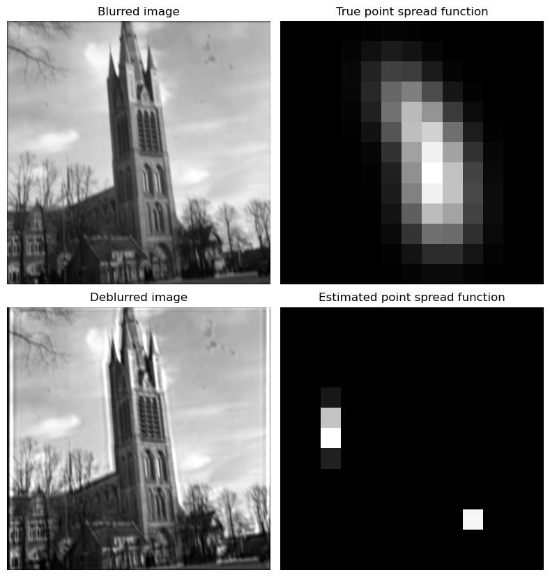
As we can see, the estimated point spread function is still far from perfect, but nevertheless the deblurred image looks better than the blurred image. If we blur the image with larger kernels, or stronger blur overall recovery becomes even harder with this method. If we apply it to a different image the result is comparable. One problem that is apparent is the fact that the point spread function tends to shift the image. This can fortunately be corrected, by either changing the point spread function or shifting the image after deconvolution.

There are probably several reasons why this model doesn’t give perfect results. First is that the image prior isn’t perfect, but it seems that most image priors tend to give quite noisy outputs, or give high scores due to artifacts created by the deconvolution algorithm. Secondly, the parameter space of this model is still quite big, especially if the prior function depends in complicated manners on these parameters. However, it seems many methods used in the literature use even larger searchspaces for the kernels, many algorithms even using no compression of the searchspace at all and still claiming good results.
While I knew from the get-go that blind deconvolution is hard, it turned out to be even harder to do right than I expected. I read a lot of literature on the subject, and I learned a lot. Many papers give interesting algorithms and ideas for blind deconvolution methods. What I found however is that most papers where quite vague in their description and almost never included code. This makes doing research in this field quite difficult, since it can be very difficult to estimate whether or not a method is actually useful. Moreover, if a method looks promising then implementing it can become very difficult without adequate details.
Other posts you may like
Rik Voorhaar © 2024