Linear algebra is the foundation of modern science, and the fact that computers can do linear algebra very fast is one of the primary reasons modern algorithms work so well in practice. In this blog post we will dive into some of the principles of fast numerical linear algebra, and learn how to solve least-squares problems using the GMRES algorithm. We apply this to the deconvolution problem, which we already discussed at length in previous blog posts.

Linear least-squares problem

The linear least-squares problem is one of the most common minimization problems we encounter. It takes the following form:

Here $A$ is an $n\times n$ matrix, and $x,b\in\mathbb R^{n}$ are vectors. If $A$ is invertible, then this problem has a simple, unique solution: $x = A^{-1}b$. However, there are two big reasons why we should almost never use $A^{-1}$ to solve the least-squares problem in practice:

1. It is expensive to compute $A^{-1}$.
2. This solution numerically unstable.

Assuming $A$ doesn’t have any useful structure, point 1. is not that bad. Solving the least-squares problem in a smart way costs $O(n^3)$, and doing it using matrix-inversion also costs $O(n^3)$, just with a larger hidden constant. The real killer is the instability. To see this in action, let’s take a matrix that is almost singular, and see what happens when we solve the least-squares problem.

import numpy as np
np.random.seed(179)

n = 20

# Create almost singular matrix
A = np.eye(n)
A[0, 0] = 1e-20
A = A @ np.random.normal(size=A.shape)

# Random vector b
b = A @ np.random.normal(size=(n,)) + 1e-3 * np.random.normal(size=n)

# Solve least-squares with inverse
A_inv = np.linalg.inv(A)
x = A_inv @ b
error = np.linalg.norm(A @ x - b) ** 2
print(f"error for matrix inversion method: {error:.4e}")


# Solve least-squares with dedicated routine
x = np.linalg.lstsq(A, b, rcond=None)[0]
error = np.linalg.norm(A @ x - b) ** 2
print(f"error for dedicated method: {error:.4e}")

Output

error for matrix inversion method: 3.6223e+02
error for dedicated method: 2.8275e-08

In this case we took a 20x20 matrix $A$ with ones on the diagonals, except for one entry where it has value

The reason that the inverse-matrix method fails badly in this case can be summarized using the condition number $\kappa(A)$. It expresses how much the error $\|Ax-b\|$ with $x=A^{-1}b$ is going to change if we change $b$ slightly, in the worst case. The condition number gives a notion of how much numerical errors get amplified when we solve the linear system. We can compute it as the ratio between the smallest and largest singular values of the matrix $A$:

In the case above the condition number is really big:

np.linalg.cond(A)

Output

1.1807555508404976e+16

Large condition numbers mean that any numerical method is going to struggle to give a good solution, but for numerically unstable methods the problem is a lot worse.

Using structure

While the numerical stability of algorithms is a fascinating topic, it is not what we came here for today. Instead, let’s revisit the first reason why using matrix inversion for solving linear problems is bad. I mentioned that matrix inversion and better alternatives take $O(n^3)$ to solve the least squares problem $\min_a\|Ax-b\|^2$, if there is no extra structure on $A$ that we can exploit.

What if there is such structure? For example, what if $A$ is a huge sparse matrix? For example the Netflix dataset we considered in this blog post is of size 480,189 x 17,769. Putting aside the fact that it is not square, inverting matrices of that kind of size is infeasible. Moreover, the inverse matrix isn’t necessarily sparse anymore, so we lose that valuable structure as well.

Another example arose in my first post on deconvolution. There we tried to solve the linear problem

where $k * x$ denotes convolution. Convolution is a linear operation, but requires only $O(n\log n)$ to compute, whereas writing it out as a matrix would require $n\times n$ entries, which can quickly become too large.

In situations like this, we have no choice but to devise an algorithm that makes use of the structure of $A$. What the two situations above have in common is that storing $A$ as a dense matrix is expensive, but computing matrix-vector products $Ax$ is cheap. The algorithm we are going to come up with is going to be iterative; we start with some initial guess $x_0$, and then improve it until we find a solution of the desired accuracy.

We don’t have much to work with; we have a vector $x_0$ and the ability fo compute matrix-vector products. Crucially, we assumed our matrix $A$ is square. This means that $x_0$ and $Ax_0$ have the same shape, and therefore we can also compute $A^2x_0$, or in fact $A^rx_0$ for any $r$. The idea is then to try to express the solution to the least-squares problem as linear combination of the vectors

This results in a class of algorithms known as Krylov subspace methods. Before diving further into how they work, let’s see one in action. We take a 2500 x 2500 sparse matrix with 5000 non-zero entries (which includes the entire diagonal).

import scipy.sparse
import scipy.sparse.linalg
import matplotlib.pyplot as plt
from time import perf_counter_ns

np.random.seed(179)

n = 2500
N = n
shape = (n, n)

# Create random sparse (n, n) matrix with N non-zero entries
coords = np.random.choice(n * n, size=N, replace=False)
coords = np.unravel_index(coords, shape)
values = np.random.normal(size=N)
A_sparse = scipy.sparse.coo_matrix((values, coords), shape=shape)
A_sparse = A_sparse.tocsr()
A_sparse += scipy.sparse.eye(n)
A_dense = A_sparse.toarray()

b = np.random.normal(size=n)
b = A_sparse @ b

# Solve using np.linalg.lstsq
time_before = perf_counter_ns()
x = np.linalg.lstsq(A_dense, b, rcond=None)[0]
time_taken = (perf_counter_ns() - time_before) * 1e-6
error = np.linalg.norm(A_dense @ x - b) ** 2
print(f"Using dense solver: error: {error:.4e} in time {time_taken:.1f}ms")

# Solve using inverse matrix
time_before = perf_counter_ns()
x = np.linalg.inv(A_dense) @ x
time_taken = (perf_counter_ns() - time_before) * 1e-6
error = np.linalg.norm(A_dense @ x - b) ** 2
print(f"Using matrix inversion: error: {error:.4e} in time {time_taken:.1f}ms")

# Solve using GMRES
time_before = perf_counter_ns()
x = scipy.sparse.linalg.gmres(A_sparse, b, tol=1e-8)[0]
time_taken = (perf_counter_ns() - time_before) * 1e-6
error = np.linalg.norm(A_sparse @ x - b) ** 2
print(f"Using sparse solver: error: {error:.4e} in time {time_taken:.1f}ms")

Output

Using dense solver: error: 1.4449e-25 in time 2941.5ms
Using matrix inversion: error: 2.4763e+03 in time 507.0ms
Using sparse solver: error: 2.5325e-13 in time 6.4ms

As we see above, the sparse matrix solver solves this problem in a fraction of the time, and the difference is just going to get bigger with larger matrices. Above we use the GMRES routine, and it is very simple. It constructs an orthonormal basis of the Krylov subspace $\mathcal K_m(A,x_0)$, and then finds the best solution in this subspace by solving a small $(m+1)\times m$ linear system. Before figuring out the details, below is a simple implementation:

def gmres(linear_map, b, x0, n_iter):
    # Initialization
    n = x0.shape[0]
    H = np.zeros((n_iter + 1, n_iter))
    r0 = b - linear_map(x0)
    beta = np.linalg.norm(r0)
    V = np.zeros((n_iter + 1, n))
    V[0] = r0 / beta

    for j in range(n_iter):
        # Compute next Krylov vector
        w = linear_map(V[j])

        # Gram-Schmidt orthogonalization
        for i in range(j + 1):
            H[i, j] = np.dot(w, V[i])
            w -= H[i, j] * V[i]
        H[j + 1, j] = np.linalg.norm(w)

        # Add new vector to basis
        V[j + 1] = w / H[j + 1, j]

    # Find best approximation in the basis V
    e1 = np.zeros(n_iter + 1)
    e1[0] = beta
    y = np.linalg.lstsq(H, e1, rcond=None)[0]

    # Convert result back to full basis and return
    x_new = x0 + V[:-1].T @ y
    return x_new

# Try out the GMRES routine
time_before = perf_counter_ns()
x0 = np.zeros(n)
linear_map = lambda x: A_sparse @ x
x = gmres(linear_map, b, x0, 50)
time_taken = (perf_counter_ns() - time_before) * 1e-6
error = np.linalg.norm(A_sparse @ x - b) ** 2
print(f"Using GMRES: error: {error:.4e} in time {time_taken:.1f}ms")

Output

Using GMRES: error: 1.1039e-15 in time 12.9ms

This clearly works; it’s not as fast as the

Let’s take a more detailed look at what the GMRES algorithm is doing. We iteratively define an orthonormal basis $V_m = \{v_0,v_1,\dots,v_{m-1}\}$. We start with $v_0 = r_0 / \|r_0\|$, where $r_0 = b-Ax_0$ is the residual of the initial guess $x_0$. In each iteration we then set $w = A v_j$, and take $v_{j+1} = w - \sum_i (w^\top v_{i})v_i$; i.e. we ensure $v_{j+1}$ is orthogonal to all previous $v_0,\dots,v_j$. Therefore $V_m$ is an orthonormal basis of the Krylov subspace $\mathcal K_m(A,r_0)$.

Once we have this basis, we want to solve the minimization problem:

Since $V_m$ is a basis, we can write $x = V_m y$ for some $y\in \mathbb R^m$. Also note that in this basis $b-Ax_0 = r_0 = \beta v_0 = \beta V_m e_1$ where $\beta = \|r_0\|$ and $e_1= (1,0,\dots,0)$. This allows us to rewrite the minimization problem:

To solve this minimization problem we need one more trick. In the algorithm we computed a matrix $H$, it is defined like this:

These are precisely the coefficients of the Gram-Schmidt orthogonalization, and hence $A v_j = \sum_{i=1}^{j+1} H_{ij}v_i$, giving the matrix equality $AV_m = HV_m$. Now we can rewrite the minimization problem even further and get

The minimization problem is therefore reduced to an $(m+1)\times m$ problem! The cost of this is $O(m^3)$, and as long as we don’t use too many steps $m$, this cost can be very reasonable. After solving for $y$, we then get the estimate $x = x_0 + V_m y$.

Restarting

In the current implementation of GMRES we specify the number of steps in advance, which is not ideal. If we converge to the right solution in less steps, then we are doing unnecessary work. If we don’t get a satisfying solution after the specified number of steps, we might need to start over. This is however not a big problem; we can use the output $x=x_0+V_my$ as new initialization when we restart.

This gives a nice recipe for GMRES with restarting. We run GMRES for $m$ steps with $x_i$ as initialization to get a new estimate $x_{i+1}$. We then check if $x_{i+1}$ is good enough, if not, we repeat the GMRES procedure for another $m$ steps.

It is possible to get a good estimate of the residual norm after each step of GMRES, not just every $m$ steps. However, this is relatively technical to implement, so we will just consider the variation of GMRES with restarting.

How often should we restart? This really depends on the problem we’re trying to solve, since there is a trade-off. More steps in between each restart will typically result in convergence in fewer steps, but it is more expensive and also requires more memory. The computational cost scales as $O(m^3)$, and the memory cost scales linearly in $m$ (if the matrix size $n$ is much bigger than $m$). Let’s see this trade-off in action on a model problem.

Deconvolution

Recall that the deconvolution problem is of the following form:

for a fixed kernel $k$ and signal $y$. The convolution operation $k*x$ is linear in $x$, and we can therefore treat this as a linear least-squares problem and solve it using GMRES. The operation $k*x$ can be written in matrix form as $Kx$, where $K$ is a matrix. For large images or signals, the matrix $K$ can be gigantic, and we never want to explicitly store $K$ in memory. Fortunately, GMRES only cares about matrix-vector products $Kx$, making this a very good candidate to solve with GMRES.

Let’s consider the problem of sharpening (deconvolving) a 128x128 picture blurred using Gaussian blur. To make the problem more interesting, the kernel $k$ used for deconvolution will be slightly different from the kernel used for blurring. This is inspired by the blind deconvolution problem, where we not only have to find $x$, but also the kernel $k$ itself.

We solve this problem with GMRES using different number of steps between restarts, and plot how the error evolves over time.

from matplotlib import image
from utils import random_motion_blur
from scipy.signal import convolve2d

# Define the Gaussian blur kernel
def gaussian_psf(sigma=1, N=9):
    gauss_psf = np.arange(-N // 2 + 1, N // 2 + 1)
    gauss_psf = np.exp(-(gauss_psf ** 2) / (2 * sigma ** 2))
    gauss_psf = np.einsum("i,j->ij", gauss_psf, gauss_psf)
    gauss_psf = gauss_psf / np.sum(gauss_psf)
    return gauss_psf


# Load the image and blur it
img = image.imread("imgs/vitus128.png")
gauss_psf_true = gaussian_psf(sigma=1, N=11)
gauss_psf_almost = gaussian_psf(sigma=1.05, N=11)
img_blur = convolve2d(img, gauss_psf_true, mode="same")


# Define the convolution linear map
linear_map = lambda x: convolve2d(
    x.reshape(img.shape), gauss_psf_almost, mode="same"
).reshape(-1)


# Apply GMRES for different restart frequencies and measure time taken
total_its = 2000
n_restart_list = [20, 50, 200, 500]
losses_dict = dict()
for n_restart in n_restart_list:
    time_before = perf_counter_ns()
    b = img_blur.reshape(-1)
    x0 = np.zeros_like(b)
    x = x0

    losses = []
    for _ in range(total_its // n_restart):
        x = gmres(linear_map, b, x, n_restart)
        error = np.linalg.norm(linear_map(x) - b) ** 2
        losses.append(error)
    time_taken = (perf_counter_ns() - time_before) / 1e9
    print(f"Best loss for {n_restart} restart frequency is {error:.4e} in {time_taken:.2f}s")
    losses_dict[n_restart] = losses

Output

Best loss for 20 restart frequency is 9.3595e-16 in 11.32s
Best loss for 50 restart frequency is 2.4392e-22 in 11.71s
Best loss for 200 restart frequency is 6.3063e-28 in 17.34s
Best loss for 500 restart frequency is 6.9367e-28 in 30.50s

We observe that with all restart frequencies we converge to a result with very low error. The larger the number of steps between restarts, the faster we converge. Remember however that the cost of GMRES rises as $O(m^3)$ with the number of steps $m$ between restarts, so a larger number of steps is not always better. For example we see that $m=20$ and $m=50$ produced almost identical runtime, but for $m=200$ the runtime for 2000 total steps is already significantly bigger, and the effect is even bigger for $m=500$. This means that if we want to get converge as fast as possible in terms of runtime, we’re best off with somewhere between $m=50$ and $m=200$ steps between each reset.

GPU implementation

If we do simple profiling, we see that almost all of the time in this function is spent on the 2D convolution. Indeed this is why the runtime does not seem to scale os $O(m^3)$ for the values of $m$ we tried above. It simply takes a while before the $O(m^3)$ factor becomes dominant over the time spent by matrix-vector products.

This also means that it should be straightforward to speed up – we just need to do the convolution on a GPU. It is not as simple as that however; if we just do the convolution on GPU and the rest of the operations on CPU, then the bottleneck quickly becomes moving the data between CPU and GPU (unless we are working on a system where CPU and GPU share memory).

Fortunately the entire GMRES algorithm is not so complex, and we can use hardware acceleration by simply translating the algorithm to use a fast computational library. There are several such libraries available for Python:

• TensorFlow
• PyTorch
• DASK
• CuPy
• JAX
• Numba

In this context CuPy might be the easiest to use; its syntax is very similar to numpy. However, I would also like to make use of JIT (Just-in-time) compilation, particularly since this can limit unnecessary data movement. Furthermore, it really depends on the situation which low-level CUDA functions are best called in different situations (especially for something like convolution), and JIT compilation can offer significant optimizations here.

TensorFlow, DASK and PyTorch are really focussed on machine-learning and neural networks, and the way we interact with these libraries might not be the best for this kind of algorithm. In fact, I tried to make an efficient GMRES implementation using these libraries, and I was really struggling; I feel these libraries simply aren’t the right tool for this job.

Numba is also great, I could basically feed it the code I already wrote and it would probably compile the function and make it several times faster on CPU. Unfortunately, the support for GPU is still lacking quite a bit in Numba, and we would therefore still leave quite a bit of performance on the table.

In the end we will implement it in JAX. Like CuPy, it has an API very similar to numpy which means it’s easy to translation. However, it also supports JIT, meaning we can potentially make much faster functions. Without further ado, let’s implement the GMRES algorithm in JAX and see what kind of speedup we can get.

import jax.numpy as jnp
import jax

# Define the linear operator
img_shape = img.shape
def do_convolution(x):
    return jax.scipy.signal.convolve2d(
        x.reshape(img_shape), gauss_psf_almost, mode="same"
    ).reshape(-1)


def gmres_jax(linear_map, b, x0, n_iter):
    # Initialization
    n = x0.shape[0]
    r0 = b - linear_map(x0)
    beta = jnp.linalg.norm(r0)
    V = jnp.zeros((n_iter + 1, n))
    V = V.at[0].set(r0 / beta)
    H = jnp.zeros((n_iter + 1, n_iter))

    def loop_body(j, pair):
        """
        One basic step of GMRES; compute new Krylov vector and orthogonalize.
        """
        H, V = pair

        w = linear_map(V[j])
        h = V @ w
        v = w - (V.T) @ h
        v_norm = jnp.linalg.norm(v)

        H = H.at[:, j].set(h)
        H = H.at[j + 1, j].set(v_norm)
        V = V.at[j + 1].set(v / v_norm)
        return H, V

    # Do n_iter iterations of basic GMRES step
    H, V = jax.lax.fori_loop(0, n_iter, loop_body, (H, V))

    # Solve the linear system in the basis V
    e1 = jnp.zeros(n_iter + 1)
    e1 = e1.at[0].set(beta)
    y = jnp.linalg.lstsq(H, e1, rcond=None)[0]

    # Convert result back to full basis and return
    x_new = x0 + V[:-1].T @ y
    return x_new


b = img_blur.reshape(-1)
x0 = jnp.zeros_like(b)
x = x0
n_restart = 50

# Declare JIT compiled version of gmres_jax
gmres_jit = jax.jit(gmres_jax, static_argnums=[0, 3])
print("Compiling function:")
%time x = gmres_jit(do_convolution, b, x0, n_restart).block_until_ready()

print("\nProfiling functions. numpy version:")
%timeit x = gmres(linear_map, b, x0, n_restart)

print("\nProfiling functions. JAX version:")
%timeit x = gmres_jit(do_convolution, b, x0, n_restart).block_until_ready()

Output

Compiling function:
CPU times: user 1.94 s, sys: 578 ms, total: 2.51 s
Wall time: 2.01 s
 
Profiling functions. numpy version:
263 ms ± 25.3 ms per loop (mean ± std. dev. of 7 runs, 1 loop each)
 
Profiling functions. JAX version:
9.16 ms ± 90.7 µs per loop (mean ± std. dev. of 7 runs, 100 loops each)

With the JAX version running on my GPU, we get a 30x times speedup! Not bad, if you ask me. If we run the same code on CPU, we still get a 4x speedup. This means that the version compiled by JAX is already faster in its own right.

The code above may look a bit strange, and there are definitely some things that might need some explanation. First of all, note that the first time we call

Note the way we create the function

    gmres_jit = jax.jit(gmres_jax, static_argnums=[0, 3])

Here we tell JAX that if the first or the fourth argument changes, the function needs to be recompiled. This is because both these arguments are python literals (the first is a function, the fourth is the number of iterations), whereas the other two arguments are arrays.

The shape of the arrays

Next, consider the fact that there is no more

    H, V = jax.lax.fori_loop(0, n_iter, loop_body, (H, V))

We could in fact use a for loop here as well, and it would give an identical result but it would take much longer to compile. The reason for this is that, as mentioned, JAX runs through the entire function and makes a graph of all the operations that need to be done. If we leave in the for loop, then each iteration of the loop would add more and more operations to the graph (the loop is ‘unrolled’), making a really big graph. By using

One disadvantage of this approach is that the size of all arrays needs to be known at compile time. In the original algorithm we did not compute

As we can see, writing code for GPUs requires a bit more thought than writing code for CPUs. Sometimes we even end up with less efficient code, but this can be entirely offset by the improved speed of the GPU.

Condition numbers and eigenvalues

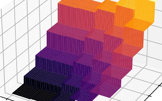
We see above that GMRES provides a very fast and accurate solution to the deconvolution problem. This has a lot to do with the fact that the convolution matrix is very well-conditioned. We can see this by looking at the singular of this matrix. The convolution matrix for a 128x128 image is a bit too big to work with, but we can see what happens for 32x32 images.

N = 11
psf = gaussian_psf(sigma=1, N=N)
img_shape = (32, 32)


def create_conv_mat(psf, img_shape):
    tot_dim = np.prod(img_shape)

    def apply_psf(signal):
        signal = signal.reshape(img_shape)
        return convolve2d(signal, psf, mode="same").reshape(-1)

    conv_mat = np.zeros((tot_dim, tot_dim))
    for i in range(tot_dim):
        signal = np.zeros(tot_dim)
        signal[i] = 1
        conv_mat[i] = apply_psf(signal)
    return conv_mat

conv_mat = create_conv_mat(psf, img_shape)
svdvals = scipy.linalg.svdvals(conv_mat)
plt.plot(svdvals)
plt.yscale('log')
cond_num = svdvals[0]/svdvals[-1]
plt.title(f"Singular values. Condition number: {cond_num:.0f}")

As we can see, the condition number is only 4409, which makes the matrix very well-conditioned. Moreover, the singular values decay somewhat gradually. What’s more, the convolution matrix is actually symmetric and positive definite. This makes the linear system relatively easy to solve, and explains why it works so well.

This is because the kernel we use – the Gaussian kernel – is itself symmetric. For a non-symmetric kernel, the situation is more complicated. Below we show what happens for a non-symmetric kernel, the same type as we used before in the blind deconvolution series of blog posts.

from utils import random_motion_blur

N = 11
psf_gaussian = gaussian_psf(sigma=1, N=N)
psf = random_motion_blur(
    N=N, num_steps=20, beta=0.98, vel_scale=0.1, sigma=0.5, seed=42
)
img_shape = (32, 32)

# plot the kernels
plt.figure(figsize=(8, 4.5))
plt.subplot(1, 2, 1)
plt.imshow(psf_gaussian)
plt.title("Gaussian kernel")
plt.subplot(1, 2, 2)
plt.imshow(psf)
plt.title("Non-symmetric kernel")
plt.show()

# study convolution matrix
conv_mat = create_conv_mat(psf, img_shape)

plt.show()
eigs = scipy.linalg.eigvals(conv_mat)
plt.title(f"Eigenvalues")
plt.ylabel("Imaginary part")
plt.xlabel("Real part")
plt.scatter(np.real(eigs), np.imag(eigs), marker=".")

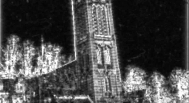
We see that the eigenvalues of this convolution matrix are distributed around zero. The convolution matrix for the gaussian kernel is symmetric and positive definite – all eigenvalues are positive real numbers. GMRES works really well when almost all eigenvalues lie in an ellipse not containing zero. That is clearly not the case here, and we in fact also see that GMRES doesn’t work well for this particular problem. (Note that we now switch to 256x256 images instead of 128x128, since our new implementation of GMRES is much faster)

img = image.imread("imgs/vitus256.png")
psf = random_motion_blur(
    N=N, num_steps=20, beta=0.98, vel_scale=0.1, sigma=0.5, seed=42
)

img_blur = convolve2d(img, psf, mode="same")
img_shape = img.shape


def do_convolution(x):
    res = jax.scipy.signal.convolve2d(
        x.reshape(img_shape), psf, mode="same"
    ).reshape(-1)
    return res


b = img_blur.reshape(-1)
x0 = jnp.zeros_like(b)
x = x0
n_restart = 1000
n_its = 10
losses = []
for _ in range(n_its):
    x = gmres_jit(do_convolution, b, x, n_restart)
    error = np.linalg.norm(do_convolution(x) - b) ** 2
    losses.append(error)

Not does it take much more iterations to converge, the final result is unsatisfactory at best. Clearly without further modifications the GMRES method doesn’t work well for deconvolution for non-symmetric kernels.

Changing the spectrum

As mentioned, GMRES works best when the eigenvalues of the matrix $A$ are in an ellipse not including zero, which is not the case for our convolution matrix. There is fortunately a very simple solution to this: instead of solving the linear least-squares problem

We solve the linear least squares problem

This will have the same solution, but the eigenvalues of $A^\top A$ are better behaved. Any matrix like this will be positive semi-definite, and all eigenvalues will be real and non-negative. They therefore all fit inside an ellipse that doesn’t include zero, and we will get much better convergence with GMRES. In general, we could multiply by any matrix $B$ to obtain the linear least-squares problem

If we choose $B$ such that the spectrum (eigenvalues) of $BA$ are nicer, then we can improve convergence of GMRES. This trick is called preconditioning. Choosing a good preconditioner depends a lot on the problem at hand, and is the subject of a lot of research. In this context, $A^\top$ turns out to function as an excellent preconditioner, as we shall see.

To apply this trick to the deconvolution problem, we need to be able to take the transpose of the convolution operation. Fortunately, this is equivalent to convolution with a reflected version $\overline k$ of the kernel $k$. That is, we will apply GMRES to the linear least-squares problem

let’s see this in action below.

img = image.imread("imgs/vitus256.png")
psf = random_motion_blur(
    N=N, num_steps=20, beta=0.98, vel_scale=0.1, sigma=0.5, seed=42
)

psf_reversed = psf[::-1, ::-1]
img_blur = convolve2d(img, psf, mode="same")
img_shape = img.shape


def do_convolution(x):
    res = jax.scipy.signal.convolve2d(x.reshape(img_shape), psf, mode="same")
    res = jax.scipy.signal.convolve2d(res, psf_reversed, mode="same")
    return res.reshape(-1)


b = jax.scipy.signal.convolve2d(img_blur, psf_reversed, mode="same").reshape(-1)
x0 = jnp.zeros_like(b)
x = x0
n_restart = 100
n_its = 20

# run once to compile
gmres_jit(do_convolution, b, x, n_restart)

time_start = perf_counter_ns()
losses = []
for _ in range(n_its):
    x = gmres_jit(do_convolution, b, x, n_restart)
    error = np.linalg.norm(do_convolution(x) - b) ** 2
    losses.append(error)
time_taken = (perf_counter_ns() - time_start) / 1e9
print(f"Deconvolution in {time_taken:.2f} s")

Deconvolution in 1.40 s

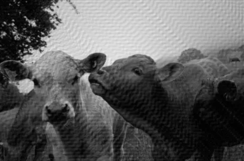
Except for some ringing around the edges, this produces very good result. Compared to other methods of deconvolution (as discussed in this blog post) this in fact shows much less ringing artifacts. It’s pretty fast as well. Even though it takes us around 2000 iterations to converge, the differences between the image after 50 steps or 2000 steps is not that big visually speaking. Let’s see how the solution develops with different numbers of iterations:

x0 = jnp.zeros_like(b)
x = x0

results_dict = {}
for n_its in [1, 5, 10, 20, 50, 100]:
    x0 = jnp.zeros_like(b)
    # run once to compile
    gmres_jit(do_convolution, b, x0, n_its)

    time_start = perf_counter_ns()
    for _ in range(10):
        x = gmres_jit(do_convolution, b, x0, n_its)
    time_taken = (perf_counter_ns() - time_start) / 1e7
    results_dict[n_its] = (x, time_taken)

After just 100 iterations the result is pretty good, and this takes just 64ms. This makes it a viable method for deconvolution, roughly equally as fast as Richardson-Lucy deconvolution, but suffering less from boundary artifacts. The regularization methods we have discussed in the deconvolution blog posts also work in this setting, and are good to use in the case where there is noise, or where we don’t precisely know the convolution kernel. That is however out of the scope of this blog post.

Conclusion

GMRES is an easy to implement, fast and robust method for solving structured linear system, where we only have access to matrix-vector products $Ax$. It is often used for solving sparse systems, but as we have demonstrated, it can also be used for solving the deconvolution problem in a way that is competitive with existing methods. Sometimes a preconditioner is needed to get good performance out of GMRES, but choosing a good preconditioner can be difficult. If we implement GMRES on a GPU it can reach much higher speeds than on CPU.