How do my music preferences evolve?
August 12, 2020
Last.fm is a great tool to keep track of the music you listen to. It’s also great for analysis!
In this article I will discuss how to download your listening history, and to annotate the data with genre information from discogs. We can then use this to track how music interests shift over time.
Where to get the data
It used to be that you can download your scrobbles straight from last.fm. Not anymore! But you can still use the API to access your scrobbles and download them this way.
Fortunately there are websites that do this for you, and just produce a .csv file of your scrobbles. I used this website , but there are alternatives.
We will be annotating the scrobbles with information about the genre. There are several music databases out there. My favorite is rateyourmusic , but it does not have an API or a way to download their database. Both discogs and MusicBrainz have a way to download frequently updated database dumps. We will be working with the discogs database, in particular the discogs_<...>_masters.xml.gz file, which contains information
about the ‘master’ releases of albums. I then used a simple script to scrape all the relevant information from this xml file, and store all the data in a simple csv file. This actually reduces the file size form 2GB down to 100MB. They also have databases with informations on artists, record labels, and individual releases of the same albums.
Importing the data
We can use pandas to read the csv files containing the scrobbles and the discogs database.
# Import the scrobble data
column_names = ['artist','album','track','date']
dtypes = {c:'str' for c in column_names}
scrobbles = pd.read_csv('scrobbles.csv', header=None, names=column_names, parse_dates=['date'], dtype=dtypes)
scrobbles.dropna(inplace=True)
scrobbles.head()| artist | album | track | date | |
|---|---|---|---|---|
| 1 | Sonic Youth | Daydream Nation | ’Cross the Breeze | 2020-08-12 15:33:00 |
| 2 | Sonic Youth | Daydream Nation | The Sprawl | 2020-08-12 15:25:00 |
| 3 | Sonic Youth | Daydream Nation | Silver Rocket | 2020-08-12 15:21:00 |
| 4 | Sonic Youth | Daydream Nation | Teen Age Riot | 2020-08-12 15:14:00 |
| 5 | Boris | Boris At Last -Feedbacker | Pt. 4 | 2020-08-12 15:01:00 |
# Import the discogs masters data
column_names = ['title','artist','year','genre','style']
masters = pd.read_csv('masters.csv', header=None, names=column_names, delimiter='\t', index_col=False)

# Convert the year entry to integer
masters.year = pd.to_numeric(masters.year, errors='coerce', downcast='integer')
masters.dropna(inplace=True)
masters.year = masters.year.astype(int)

# Sort by artist - album title
masters.sort_values(by=['artist','title'], inplace=True)
masters.reset_index(drop=True, inplace=True)

masters.head()| title | artist | year | genre | style | |
|---|---|---|---|---|---|
| 0 | Twenty Four- Twenty Five | ! Z-Loc | 1996 | Hip Hop | Jazzy Hip-Hop |
| 1 | !!! | !!! | 2000 | Electronic | Leftfield;Experimental;Disco |
| 2 | AM/FM | !!! | 2010 | Electronic;Rock | Indie Rock;Disco |
| 3 | All U Writers / Gonna Guetta Stomp | !!! | 2015 | Electronic;Rock | House |
| 4 | And Anyway It’s Christmas | !!! | 2013 | Rock | Punk;Pop Punk |
Global listening history
The first thing we can look at is how much music I listened since I started using last.fm. We can see some interesting patterns here. For example back in high school I used to spend much more time listening to music than I do nowadays. There is also a dip in the Fall of 2014, when I was in Japan for a few months. The dip at the start of 2016 coincides with the time I started to date my wife. It’s also interesting to note that since the start of Coronavirus measures I have been listening to music much more as well.
import matplotlib.dates as mdates
import matplotlib.ticker as mtick
from scipy.ndimage import gaussian_filter1d

# Find the number of scrobbles on each individual day
# This does not include any days wihtout scrobbles
date_density = pd.Series(1,index=scrobbles.date).resample('D').sum()

# Make a day range encompassing scrobbles' dates
start_day = date_density.index[0].strftime('%Y-%m-%d')
end_day = date_density.index[-1].strftime('%Y-%m-%d')
date_range = pd.date_range(start=start_day,end=end_day,freq='D')

# Make a series containing number of scrobbles for each day in range
all_days = pd.Series(0,index=date_range)
all_days[date_density.index] = date_density

# Apply a gaussian filter to smoothen the timeseries
all_days.iloc[:] = gaussian_filter1d(all_days.values.astype(float), sigma=30)

# Plot the data
plt.figure(figsize=(16,5))
plt.plot(all_days)
plt.title('Average daily scrobbles over time (gaussian filter, sigma=30d)')
plt.ylabel('Number of daily scrobbles')
ax = plt.gca()
ax.xaxis.set_major_locator(mdates.YearLocator() )
ax.xaxis.set_major_formatter(mdates.DateFormatter('%Y'))
ax.xaxis.set_minor_locator(mdates.MonthLocator() )
plt.show()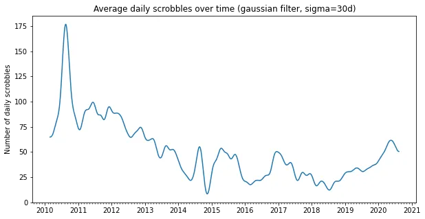
Annotating the scrobbles
What we want to do next is to annotate the scrobbles with genre information. We will first of all create an index which maps the title of an album to the row index in the discogs dataframe. Unfortunately the titles of albums don’t always match up exactly between the scrobbles and the discogs database. We can improve this slightly by preprocessing the titles of the albums slightly, but this can still be improved further.
from collections import defaultdict

def prepare_album_title(title):
    return title.split('(')[0][:50].lower()

# Make index mapping album titles to row numbers
album_index = defaultdict(list)
for i, title in masters.title.iteritems():
    album_index[prepare_album_title(title)].append(i)
Now we will look up the genre information for all the scrobbles. For each different genre we will make a timeseries of scrobbles, so that we can see how my preference of specific genres evolves over time.
import functools

# Cache results, since we will be looking up the same album many times.
@functools.lru_cache(maxsize=None)
def get_styles(album, artist=None):
    """Look up a list of genres for an album-artist combination."""
    # Look up the album title in the masters dataframe
    title = prepare_album_title(album)
    index = album_index.get(title,[])
    df_slice = masters.loc[index]

    # Only pick the albums that match the artist
    if artist is not None and len(df_slice)>2:
        artists = (df_slice['artist'].str.lower()).str.slice(stop=10)
        mask = artists.str.startswith(artist.lower()[:10])
        df_slice = df_slice[mask]

    # If there are no hits, return empty set
    if len(df_slice) == 0:
        return set()

    # For each result, look up the genre, and return as set
    styles = set((';'.join(df_slice['style'])).split(';'))
    return styles

# Look up genre information for each scrobble
# Save the date of the scrobble in a seperate list for each genre
styles_dic = defaultdict(list)
for row in tqdm(scrobbles.itertuples(), total=len(scrobbles)):
    styles = get_styles(row.album,row.artist)
    for style in styles:
        styles_dic[style].append(row.date)
Now that we have a time series for each genre, let’s first of all look what the most common genres are.
sorted([(key,len(item)) for key,item in styles_dic.items()],key=lambda x:-x[1])[:10]Output
[(‘Alternative Rock’, 30936), (‘Indie Rock’, 22703), (‘Pop Rock’, 20226), (‘Psychedelic Rock’,
14917), (‘Experimental’, 13524), (‘Rock & Roll’, 13502), (‘Stoner Rock’, 11381), (‘Industrial’,
10592), (‘Hard Rock’, 9145), (‘Prog Rock’, 9035)]
Now finally let’s look at how my listening preferences evolve over time. We will write a function that plots a timeseries for a particular genre. Like with the global scrobble data, we will be smoothing this with a gaussian kernel.
def plot_genre(genre):
    # Get the daily counts for this genre
    day_counts = pd.Series(1,index=styles_dic[genre]).resample('D').sum()

    # Make a timeseries
    all_counts = pd.Series(0,index=all_days.index)
    all_counts[day_counts.index] = day_counts

    # Smoothen with gaussian filtern and turn into percentage
    all_counts.iloc[:] = 100*gaussian_filter1d(all_counts.values.astype(float), sigma=30)/all_days.values

    # Plot the data
    plt.figure(figsize=(16,5))
    plt.plot(all_counts)
    ax = plt.gca()

    ax.xaxis.set_major_locator(mdates.YearLocator() )
    ax.xaxis.set_major_formatter(mdates.DateFormatter('%Y'))
    ax.xaxis.set_minor_locator(mdates.MonthLocator() )
    ax.yaxis.set_major_formatter(mtick.PercentFormatter())

    plt.ylabel('Percentage of listens tagged with genre')
    plt.title(f'Average daily scrobbles of {genre}')
    plt.show()
Results
Unfortunately, a lot of the genres are not very descriptive, so not all of the timeseries are very informative, but there are some with interesting patters showing how my tastes really change over time. I could come up with some ‘eras’ describing my predominant genres over some time periods, but of course there is a lot of overlap.
2010-2012: Pop Rock
I used to listen to the Beatles a lot back in high school, and that’s clearly reflected on this graph. Later on this mostly subsided, and while I still love the Beatles, I can’t say I often feel like listening to them anymore.
plot_genre('Pop Rock')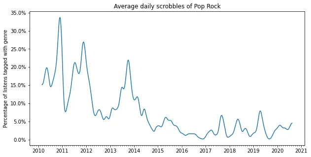
2012: J-pop
Around 2012 I got infatuated with Tokyo Jihen and Ringo Shiina’s music, as well as some other J-pop. Interstingly, by the time I was actually living in Japan for a bit, my obsession had already mostly left me.
plot_genre('J-pop')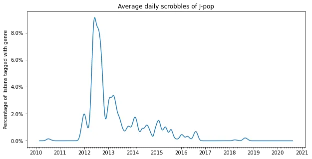
2011-2013 Prog Rock
Starting in the two lastyears of high school I had a long period where I listened to a lot of prog rock. This was mostly dominated by King Crimson, and for a long while I considered King Crimson to be my favorite band.
plot_genre('Prog Rock')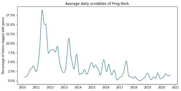
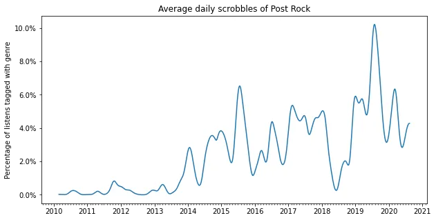
2015 - 2020: Noise and post rock
From roughly 2015 onward I started listening to more noisy and experimental music. I also discovered the magic of post-rock with bands such as Godspeed You! Black Emperor and Slint. I think this is around the time that I started to realize that for me the texture of music is more important than the lyrics or melody.
plot_genre('Noise')
plot_genre('Post Rock')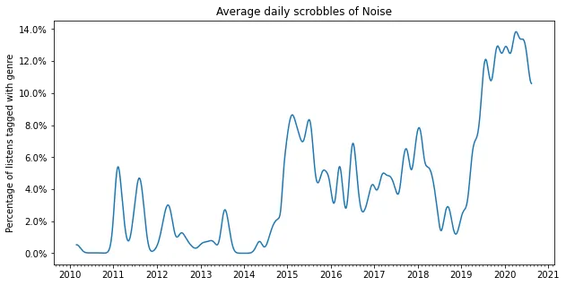
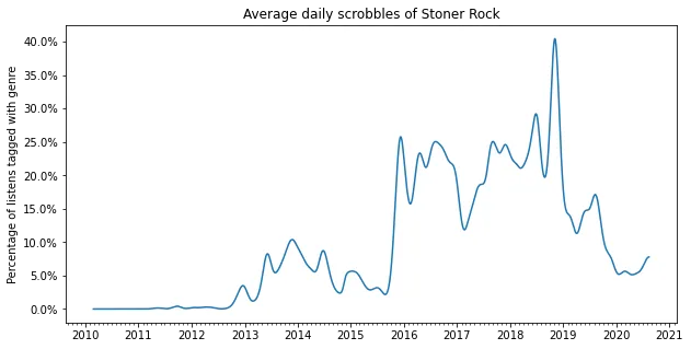
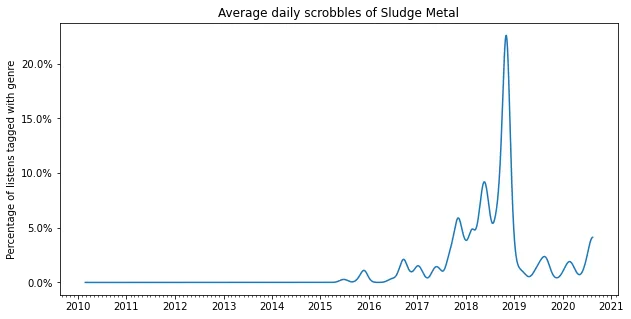
2016-2019: Stoner/Doom
In 2016 I discovered stoner rock and doom metal. Before this I was occasionally listening to Boris since 2013, but it never really stuck. Then suddenly I discovered a lot of stoner rock on youtube, and I became hooked. Lately I haven’t been listening to it as much, but I still consider Melvins and Boris to be my favorite bands.
plot_genre('Doom Metal')
plot_genre('Stoner Rock')
plot_genre('Sludge Metal')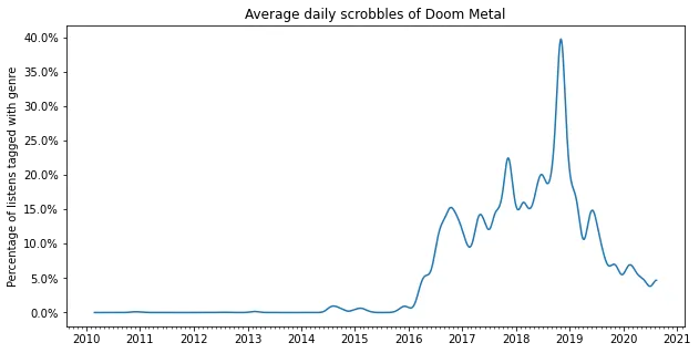
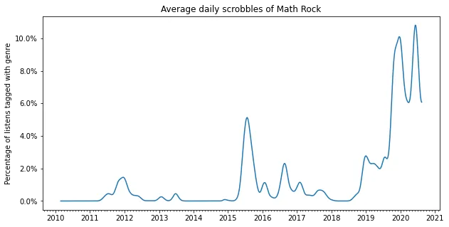
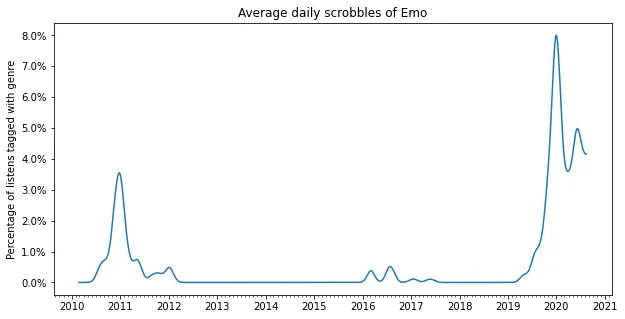
2020: Punk, math rock and emo
My most recent obsession has become punk and emo, the noisier the better. I really like the noisy texture, and have fallen in love with bands such as Polvo, Drive Like Jehu and Shellac. At the same time I also discovered some great punk bands like Idles, Parquet Courts and (very recently) Jeff Rosenstock.
plot_genre('Punk')
plot_genre('Math Rock')
plot_genre('Emo')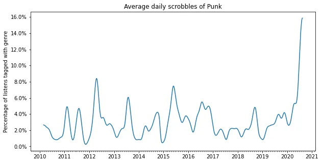
What’s next?
There are still many fascinating things I would love to do with my listening data. One thing I would really love to try is to cluster artists based on the timeseries of scrobbles, e.g. base distance between artists on the time distance between listening to them. This might very well correspond to a rough genre clustering.
Keep reading

7th of October, 2023
In my first dive into Rust, I implemented an unscented Kalman filter in and made it 20x faster than the equivalent Python implementation.
1st of May, 2023
I made an interactive dashboard for this website, and here is the story of how I did it.

13th of February, 2021
I have 15 years worth of email traffic data, let's take a closer look and discover some fascinating patterns.

9th of November, 2020
We use exams to determine how much a student knows, but exams aren't perfect. How can we estimate the uncertainty in students' exams scores?
26th of August, 2020
Cross validation is extremely important, but how should we choose the size of our validation and test sets?
10th of August, 2020
Normally distributed data is great, but how do you know whether your data is normally distributed?

20th of June, 2020
Judging in figure skating is biased. Let's use data science to figure out just how bad the issue is.

15th of January, 2025
I made an array programming language as a language extension to Rust

1st of August, 2024
Self-hosting your own cloud services not only saves money, it is also a great way to learn

26th of February, 2023
Read this blog post if you're curious what I worked on during my PhD!
29th of March, 2022
Linear least-squares system pop up everywhere, and there are many fast way to solve them. We'll be looking at one such way: GMRES.
10th of March, 2022
We recently made a paper about supervised machine learning using tensors, here's the gist of how this works.
26th of September, 2021
A lot of data is naturally of 'low rank'. I will explain what this means, and how to exploit this fact.
29th of August, 2021
Parsing and editing Word documents automatically can be extremely useful, but doing it in Python is not that straightforward.

31st of May, 2021
Finally, let's look at how we can automatically sharpen images, without knowing how they were blurred in the first place.

2nd of May, 2021
Deconvolving and sharpening images is actually pretty tricky. Let's have a look at some more advanced methods for deconvolution.

9th of April, 2021
In order to automatically sharpen images, we need to first understand how a computer can judge how 'natural' an image looks.

13th of March, 2021
Deconvolution is one of the cornerstones of image processing. Let's take a look at how it works.