A few months ago, I defended my thesis and earned the title of “doctor.” I’m excited to share the contents of my thesis defense with you in this blog post, where you can get a glimpse of the fascinating research I conducted over the past few years. The post is divided into several parts, with the level of technical detail increasing gradually.

If you’re interested in reading my full thesis, you can find it here. I’ve also made my defense slides available for download here.

Low-rank matrices

My thesis focuses on low-rank tensors, but to understand them, it’s important to first discuss low-rank matrices. You can learn more about low-rank matrices in this blog post. A low-rank matrix is simply the product of two smaller matrices. For example below we write the matrix $A$ as the product $A=XY^\top$.

In this case, the matrix $X$ is of size $m\times r$ and the matrix $Y$ is of size $n\times r$. This usually means that the product $A$ is a rank-$r$ matrix, though it could have a lower rank if for example one of the rows of $X$ or $Y$ is zero.

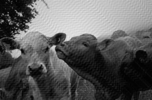
While many matrices encountered in real-world applications are not low-rank, they can often be well approximated by low-rank matrices. Images, for example, can be represented as matrices (if we consider each color channel separately), and low-rank approximations of images can give recognizable results. In the figure below, we can see several low-rank approximations of an image, with higher ranks giving better approximations of the original image.

To determine the “best” rank-$r$ approximation of a matrix $A$, we can solve the following optimization problem:

There are several ways to solve this approximation problem, but luckily in this case there is a simple closed-form solution known as the truncated SVD. To apply this method using numpy, we can use the following code:

def low_rank_approx(A, r):
    U, S, Vt = np.linalg.svd(A)
    return U[:, :r] @ np.diag(S[:r]) @ Vt[:r, :]

One disadvantage of this particular function is that it hides the fact that the output has rank $\leq r$, since we’re just returning an $m\times n$ matrix. However, we can fix this easily as follows:

def low_rank_approx(A, r):
    U, S, Vt = np.linalg.svd(A)
    X = U[:, :r] @ np.diag(S[:r])
    Y = Vt[:r, :].T
    return X, Y

Low-rank matrices are computationally efficient because they enable fast products. If we have two large $n\times n$ matrices, it takes $O(n^3)$ flops to compute their product using conventional matrix multiplication algorithms. However, if we can express the matrices as low-rank products, such as $A=X_1Y_1^\top$ and $B=X_2Y_2^\top$, then computing their product requires only $O(rn^2)$ flops. Even better, the product can be expressed as the product of two $n\times r$ matrices using only $O(r^2n)$ flops, which is potentially much less than $O(n^3)$. Similarly, if we want to multiply a matrix with a vector, a low-rank representation can greatly reduce the computational cost.

Matrix completion

The decomposition of a size $m\times n$ matrix $A$ into $A=XY^\top$ uses only $r(m+n)$ parameters, compared to the $mn$ parameters required for the full matrix. (In fact, due to symmetry, we only need $r(m+n) - r^2$ parameters.) This implies that with more than $r(m+n)$ entries of the matrix known, we can infer the remaining entries of the matrix. This is called matrix completion, and we can achieve it by solving an optimization problem, such as:

where $\Omega$ is the set of known entries of $A$, and $\mathcal P_\Omega$ is the projection that sets all entries in a matrix not in $\Omega$ to zero.

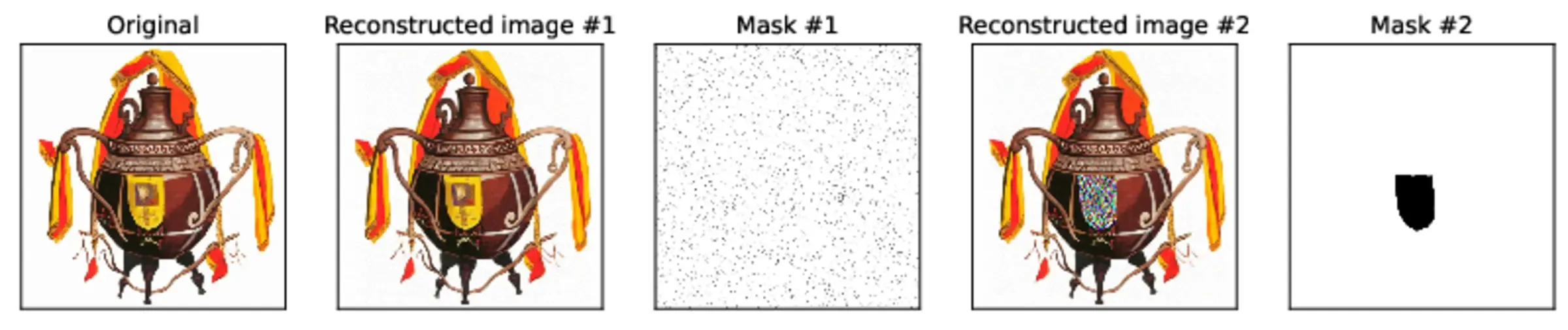
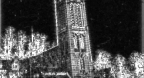
Matrix completion is illustrated in two examples of reconstructing an image as a rank 100 matrix, where 2.7% of the pixels were removed. The effectiveness of matrix completion depends on the distribution of the unknown pixels. When the unknown pixels are spread out, matrix completion works well, as seen in the first example. However, when the unknown pixels are clustered in specific regions, matrix completion does not work well, as seen in the second example.

There are various methods to solve the matrix completion problem, and one simple technique is alternating least squares optimization, which I also discussed in this blog post. This approach optimizes the matrices $X$ and $Y$ alternately, given the decomposition $B=XY^\top$. Another interesting method is solving a slightly different optimization problem which turns out to be convex, which can thus b solved using the machinery of convex optimization. Another effective method is Riemannian gradient descent, which is also useful for low-rank tensors. The idea is to treat the set of low-rank matrices as a Riemannian manifold, and then use gradient descent methods. The gradient is projected onto the tangent space of the manifold, and then a step is taken in the projected direction, which keeps us closer to the constraint set. The projection back onto the manifold is usually cheap to compute, and can be combined with the step into a single operation known as a retraction. The challenge of Riemannian gradient descent is to find a retraction that is both cheap to compute and effective for optimizing the objective.

Low-rank tensors

Let’s now move on to the basics of tensors. A tensor is a multi-dimensional array, with a vector being an order 1 tensor and a matrix being an order 2 tensor. An order 3 tensor can be thought of as a collection of matrices or an array whose entries can be represented by a cube of values. Unfortunately, this geometric way of thinking about tensors breaks down at higher orders, but in principle still works.

Some examples of tensors include:

• Order 1 (vector): Audio signals, stock prices
• Order 2 (matrix): Grayscale images, excel spreadsheets
• Order 3: Color images, B&W videos, Minecraft maps, MRI scans
• Order 4: Color video, fMRI scans

Recall that a matrix is low-rank if it is the product of two smaller matrices, that is, $A=XY^\top$. Unfortunately, this notation doesn’t generalize well to tensors. Instead, we can write down each entry of $A$ as a sum:

Similarly, we could write an order 3 tensor as a product of 3 matrices as follows:

However, if we’re dealing with more complicated tensors of higher order, this kind of notation can quickly become unwieldy. One way to get around this is to use a diagrammatic notation, where tensors are represented by boxes with one leg (edge) for each of the tensor’s indices. Connecting two boxes via one of these legs denotes summation over the associated index. For example, matrix multiplication is denoted as follows:

To make it clearer which legs can be contracted together, it’s helpful to label them with the dimension of the associated index; it is only possible to sum over an index belonging to two different tensors if they have the same dimension.

We can for example use the following diagram to depict the low-rank order 3 tensor described above:

In this case, we sum over the same index for three different matrices, so we connect the three legs together in the diagram. This resulting low-rank tensor is called a “CP tensor”, where “CP” stands for “canonical polyadic”. This tensor format can be easily generalized to higher order tensors. For an order-d tensor, we can represent it as:

The CP tensor format is a natural generalization of low-rank matrices and is straightforward to formulate. However, finding a good approximation of a given tensor as a CP tensor of a specific rank can be difficult, unlike matrices where we can use truncated SVD to solve this problem. To overcome this limitation, we can use a slightly more complex tensor format known as the ”tensor train format” (TT).

Tensor trains

Let’s consider the formula for a low-rank matrix decomposition once again: $A=C_1C_2$

We can express this as follows:

Alternatively, we can rewrite this as the product of row $i_1$ of the first matrix and column $i_2$ of the second matrix, like so: $A[i_1,i_2] = C_1[i_1,:]C_2[:,i_2]$ This can be visualized as follows:

To extend this to an order-3 tensor, we can represent $A[i_1,i_2,i_3]$ as the product of 3 vectors, which is known as the CP tensor format. Alternatively, we can express $A[i_1,i_2,i_3]$ as a vector-matrix-vector product, like so:

This can be represented visually as shown below:

Extending this to an arbitrary order is straightforward. For example, for an order-4 tensor, we would write each entry of the tensor as a vector-matrix-matrix-vector product, like so:

which can be depicted like this:

Let’s translate the formula back into diagrammatic notation. We want to represent an order 4 tensor as a box with four legs, expressed as the product of a matrix, two order 3 tensors, and another matrix. This is the resulting diagram:

An arbitrary tensor train can be denoted as follows:

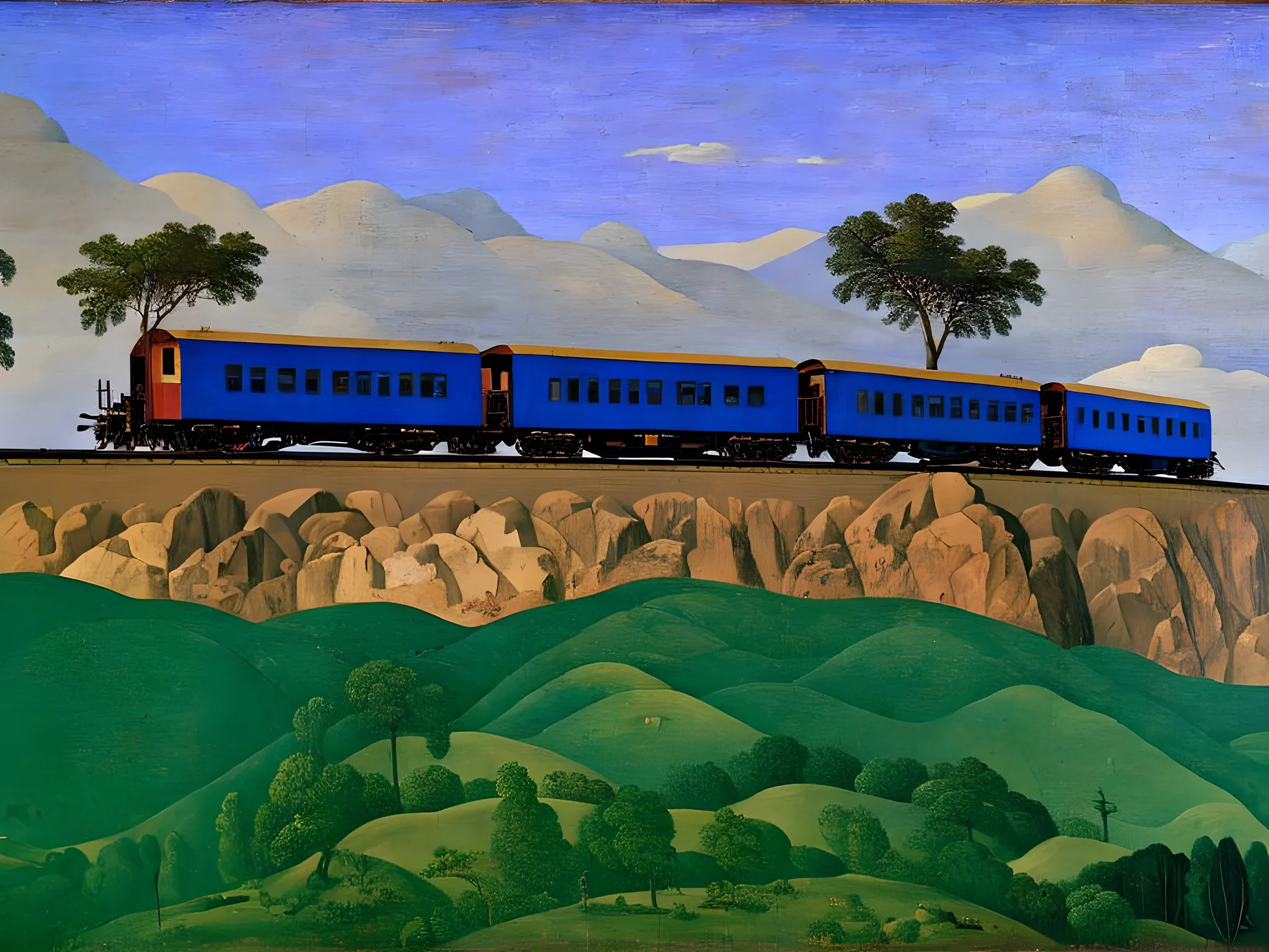
This notation helps us understand why this decomposition is called a tensor train. Each box of order 2/3 tensors represents a “carriage” in the train. We can translate the above diagram into a train shape, like this:

Although I am not skilled at drawing, we can use stable diffusion to create a more aesthetically pleasing depiction:

Tensor trains: what are they good for?

From what we have seen so far it is not obvious what makes the tensor train decomposition such a useful tool. Although these properties are not unique to the tensor train decomposition, here are some reasons why it is a good decomposition for many applications.

Computing entries is fast: Computing an arbitrary entry $A[i_1,\dots,i_d]$ is very fast, requiring just a few matrix-vector products. These operations can be efficiently done in parallel using a GPU as well.

Easy to implement: Most algorithms involving tensor trains are not difficult to implement, which makes them easier to adopt. A similar tensor decomposition known as the hierarchical tucker decomposition is much more tricky to use in practical code, which is likely why it is less popular than tensor trains despite theoretically being a superior format for many purposes.

Dimensional scaling: If we keep the ranks $r = r_1=\dots=r_{d-1}$ of an order-$d$ tensor train fixed, then the amount of data required to store and manipulate a tensor train only scales linearly with the order of the tensor. A dense tensor format would scale exponentially with the tensor order and quickly become unmanageable, so this is an important property. Another way to phrase this is that tensor trains do not suffer from the curse of dimensionality.

Orthogonality and rounding: Tensor trains can be orthogonalized with respect to any mode. They can also be rounded, i.e. we can lower all the ranks of the tensor train. These two operations are extremely useful for many algorithms and have a reasonable computational cost of $O(r^3nd)$ flops, and are also very simple to implement.

Nice Riemannian structure: The tensor trains of a fixed maximum rank form a Riemannian manifold. The tangent space, and orthogonal projections onto this tangent space, are relatively easy to work with and compute. The manifold is also topologically closed, which means that optimization problems on this manifold are well-posed. These properties allow for some very efficient Riemannian optimization algorithms.

Using tensor trains for machine learning

With the understanding that low-rank tensors can effectively represent discretized functions, I will demonstrate how tensor trains can be utilized to create a unique type of machine learning estimator. To avoid redundancy, I will provide a condensed summary of the topic, and I invite you to read my more detailed blog post on this subject if you would like to learn more.

Matrices as discretized functions

Let’s consider a function $f(x,y)\colon I^2\to \mathbb R$ and plot its values on a square. For instance, we can use the following function:

Note that grayscale images can be represented as matrices, so if we use $m\times n$ pixels to plot the function, we get an $m\times n$ matrix. Surprisingly, this matrix is always rank-4, irrespective of its size. We illustrate the rows of matrices $X$ and $Y$ of the low-rank decomposition $A=XY^\top$ below. Notice that increasing the matrix size doesn’t visibly alter the low-rank decomposition.

This suggests that low-rank matrices can potentially capture complex 2D functions. We can extend this to higher dimensions by using low-rank tensors to represent intricate functions.

We can use low-rank tensors to parametrize complicated functions using relatively few parameters, which makes them suitable as a supervised learning model. Suppose we have a few samples $y_j = \hat f(x_j)$ with $j=1,\dots, N$ for $x_j\in\mathbb R^{d}$, where $\hat f$ is an unknown function. Let $f_A$ be the discretized function obtained from a tensor or matrix $A$. We can formulate supervised learning as the following least-squares problem:

Each data point $x_j$ corresponds to an entry $A[i_1(x_j),\dots,i_d(x_j)]$, which allows us to rephrase the least-squares problem as a matrix/tensor completion problem.

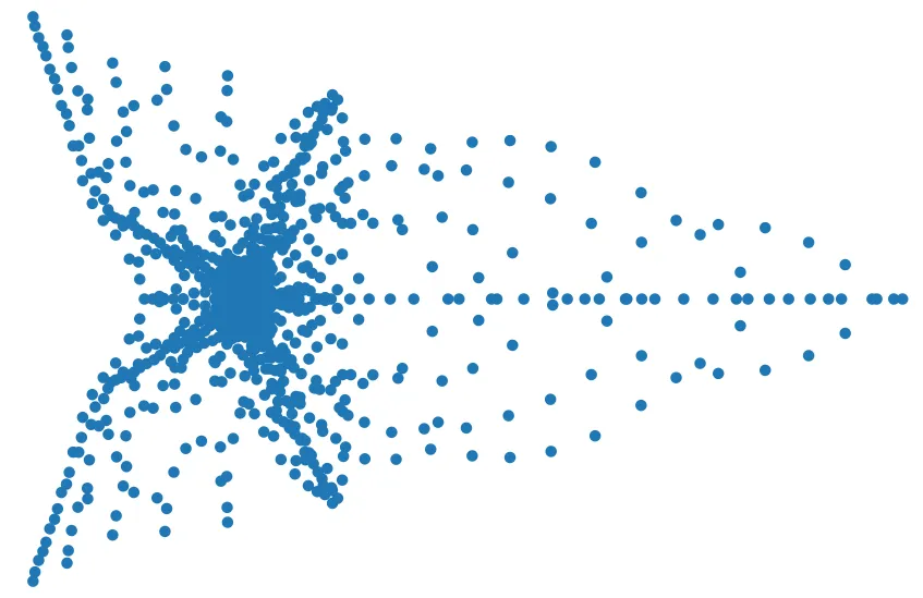
Let’s see this in action for the 2D/matrix case to gain some intuition. First, let’s generate some random points in a square and sample the function $f(x,y)$ defined above. On the left, we see a scatterplot of the random value samples, and next, we see what this looks like as a discretized function/matrix.

If we now apply matrix completion to this, we get the following. First, we see the completed matrix using a rank-8 matrix, and then the matrices $X, Y$ of the decomposition $A=XY^\top$.

What we have so far is already a useable supervised learning model; we plug in data, and as output, it can make reasonably accurate predictions of data points it hasn’t seen so far. However, the data used to train this model is uniformly distributed across the domain. Real data is rarely like that, and if we plot the same for images for less uniformly distributed data the result is less impressive:

How can we get around this? Well, if the data is not uniform, then why should we use a uniform discretization? For technical reasons, the discretization is still required to be a grid, but we can adjust the spacing of the grid points to better match the data. If we do this, we get something like this:

While the final function (3rd plot) may look odd, it does achieve two important things. First, it makes the matrix-completion problem easier because we start with a matrix where a larger percentage of entries are known. And secondly, the resulting function is accurate in the vicinity of the data points. So long as the distribution of the training data is reasonably similar to the test data, this means that the model is accurate on most test data points. The model is potentially not very accurate in some regions, but this may simply not matter in practice.

TT-ML

Now, let’s dive into the high-dimensional case and examine how tensor trains can be employed for supervised learning. In contrast to low-rank matrices, we will utilize tensor trains to parameterize the discretized functions. This involves solving an optimization problem of the form:

where $\mathscr M$ denotes the manifold of all tensor trains with a given maximum rank. To tackle this optimization problem effectively, we can use the Riemannian structure of the tensor train manifold. This approach results in an optimization algorithm similar to gradient descent (with line search) but utilizing Riemannian gradients instead.

Unfortunately, the problem $(\star)$ is very non-linear and the objective has many local minima. As a result, any gradient-based method will only produce good results if it has a good initialization. The ideal initialization is a tensor that describes a discretized function with low training/test loss. Fortunately, we can easily obtain such tensors by training a different machine learning model (such as a random forest or neural network) on the same data and then discretizing the resulting function. However, this gives us a dense tensor, which is impractical to store in memory. We can still compute any particular entry of this tensor cheaply, equivalent to evaluating the model at a point. Using a technique called TT-cross, we can efficiently obtain a tensor-train approximation of the discretized machine learning model, which we can then use as initialization for the optimization routine.

But why go through all this trouble? Why not just use the initialization model instead of the tensor train? The answer lies in the speed and size of the resulting model. The tensor train model is much smaller and faster than the model it is based on, and accessing any entry in a tensor train is extremely fast and easy to parallelize. Moreover, low-rank tensor trains can still parameterize complicated functions.

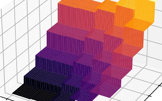
To summarize the potential advantages of TTML, consider the following three graphs (for more details, please refer to my thesis):

Based on the results shown in the graphs, it is clear that the TTML model has a significant advantage over other models in terms of size and speed. It is much smaller and faster than other models while maintaining a similar level of test error. However, it is important to note that the performance of the TTML model may depend on the specific dataset used, and in many practical machine learning problems, its test error may not be as impressive as in the experiment shown. That being said, if speed is a crucial factor in a particular application, the TTML model can be a very competitive option.

Randomized linear algebra

As we have seen above, the singular value decomposition (SVD) can be used to find the best low-rank approximation of any matrix. Unfortunately, the SVD is rather expensive to compute, costing $O(mn^2)$ flops for an $m\times n$ matrix. Moreover, while SVD can also be used to compute good low-rank TT approximations of any tensor, the cost of the SVD can become prohibitively expensive in this context. Therefore, we need a faster way to compute low-rank matrix approximations.

In my blog post I discussed some iterative methods to compute low-rank approximations using only matrix-vector products. However, there are even faster non-iterative methods that are based on multiplying the matrix of interest with a random matrix.

Specifically, if $A$ is a rank-$\hat r$ matrix of size $m\times n$ and $x$ is a random matrix of size $r>\hat r$, then it turns out that the product $AX$ almost always has the same range as $A$. This is because multiplying by $X$ like this doesn’t change the rank of $A$ unless $X$ is chosen adversarially. However, since we assume $X$ is chosen randomly this almost never happens. And here ‘almost never’ is meant in the mathematical sense – i.e., with probability zero. As a result, we have the identity $\mathcal P_{AX}A =A$, where $\mathcal P_{AX}$ denotes the orthogonal projection onto $AX$. This projection matrix can be computed using the QR decomposition of $AX$, or it can be seen simply as the matrix whose columns form an orthogonal basis of the range of $AX$.

If $A$ has rank $\hat r>r$ however, then $\mathcal P_{AX}A\neq A$. Nevertheless, we might hope that these two matrices are close, i.e. we may hope that (with probability 1) we have

for some constant $C$ that depends only on $\hat r$ and the dimensions of the problem. Recall that here $A_{\hat r}$ denotes the best rank-$\hat r$ approximation of $A$ (which we can compute using the SVD). It turns out that this is true, and it gives a very simple algorithm for computing a low-rank approximation of a matrix using only $O(mnr)$ flops – a huge gain if $r$ is much smaller than the size of the matrix. This is known as the Halko-Martinsson-Tropp (HMT) method, and can be implemented in Python like this:

def hmt_approximation(A, r):
    m, n = A.shape
    X = np.random.normal(size=(n, r))
    AX = A @ X
    Q, _ = np.linalg.qr(AX)
    return Q, Q.T @ A

Since $Q(Q^\top A) = \mathcal P_{AX}A$, this gives a low-rank approximation. It can also be used to obtain an approximate truncated SVD with a minor modification: if we take the SVD $U\Sigma V^\top = Q^\top A$, then $(QU)\Sigma V^\top$ is an approximate truncated SVD of $A$. In Python we could implement this like this:

def hmt_truncated_svd(A, r):
    Q, QtA = hmt_approximation(A, r)
    U, S, Vt = np.linalg.svd(QtA)
    return Q @ U, S, Vt

The HMT method, while efficient, has some drawbacks compared to other randomized methods. For instance, it cannot compute a low-rank decomposition of the sum $A+B$ of two matrices in parallel since the QR decomposition of $(A+B)X$ requires the computation of $(A+B)X$ first. Additionally, if a low-rank approximation $Q(Q^\top A)$ has already been computed and a small change $B$ is made to $A$ to obtain $A' = A + B$, it is not possible to compute an approximation of the same rank for $A'$ without redoing most of the work.

The issue arises from the fact that computing a QR decomposition of the product $AX$ is nonlinear and expensive. One way to address this is by introducing a second random matrix $Y$ of size $m\times r$ and computing a decomposition of $Y^\top AX$. This matrix has a much smaller size of $r\times r$, allowing for efficient computations if $r$ is small. Furthermore, computing $Y^\top(A+B)X$ can be performed entirely in parallel. This results in a low-rank decomposition of the form:

where $\dagger$ denotes the pseudo-inverse. This is a generalization of the matrix inverse to non-invertible or rectangular matrices, and it can be computed using the SVD of a matrix. If $A=U\Sigma V^\top$, then $A^\dagger = V\Sigma^{-1} U^\top$. To compute the inverse of $\Sigma$, we set $\Sigma^{-1}[i,i] = 1/(\Sigma[i,i])$ unless one of the diagonal entries is zero, in which case it remains untouched.

The randomized decomposition we discussed is known by different names and has appeared in slightly different forms many times in the literature. In my thesis, I refer to it as the “generalized Nyström” (GN) method. Like the HMT method, it is “quasi-optimal”, which means that it satisfies:

However, there are two technical caveats that need to be discussed. The first is that if we need to choose X and Y to be of different sizes; that is, we must have X of size $m \times r_R$ and Y of size $n \times r_L$ with $r_L \neq r_R$. This is because otherwise $(Y^\top AX)^\dagger$ can have strange behavior. For example, the expected spectral norm $\mathbb{E} \|(Y^\top AX)^\dagger\|_2$ is infinite if $r_L=r_R$.

The second caveat is that explicitly computing $(Y^\top AX)^\dagger$ and then multiplying it by $AX$ and $Y^\top A$ can lead to numerical instability. However, a product of the form $A^\dagger B$ is equivalent to the solution of a linear problem of the form $AX=B$. As a result, we could implement this method in Python as follows:

def generalized_nystrom(A, rank_left, rank_right):
    m, n = A.shape
    X = np.random.normal(size=(n, rank_right))
    Y = np.random.normal(size=(m, rank_left))
    AX = A @ X
    YtA = Y.T @ A
    YtAX = Y.T @ AX
    L = YtA
    R = np.linalg.solve(YtAX, AX, rcond=None)
    return L, R

Note that this method computes the decomposition implicitly by solving a linear system of equations, which is more stable and efficient than explicitly computing the pseudo-inverse.

Randomized tensor train approximations

Next, we will see how to generalize the GN method to a method for tensor trains. Unfortunately this will get a little technical. Recall that for the GN decomposition we had a decomposition of form

To generalize the GN method to the tensor case, we can take a matricization of the tensor $\mathcal{T}$ with respect to a mode $\mu$, which gives a matrix $\mathcal{T}^{\leq \mu}$ of size $(n_1 \cdots n_\mu) \times (n_{\mu+1} \cdots n_d)$. We can then multiply this matrix on the left and right with random matrices $Y_\mu$ and $X_\mu$ of size $(n_1 \cdots n_\mu) \times r_L$ and $(n_{\mu+1} \cdots n_d) \times r_R$, respectively, to obtain the product

We call this product a ‘sketch’, and this particular sketch corresponds to the product $Y^\top AX$ in the matrix case. We visualize the computation of this sketch below:

If we think of a matrix as a tensor with only two modes (legs), then the products $AX$ and $Y^\top A$ correspond to multiplying the tensor by matrices such that ‘one mode is left alone’. From this perspective, we can generalize these products to the sketch

where $Y_{\mu-1}$ is now a matrix of size $(n_1\dots n_{\mu-1})\times r_L$, also depicted below:

By extension, we can define $Y_0=X_d=1$, and then the definition of $\Psi_\mu$ reduces to $\Psi_1=AX$ and $\Psi_2=Y^\top A$ in the matrix case. We can therefore rewrite the GN method as

More generally, we can chain the sketches $\Omega_\mu$ and $\Psi_\mu$ together to form a tensor network of the following form:

With only minor work, we can turn this tensor network into a tensor train. It turns out that this defines a very useful approximation method for tensor trains. However, it may not be immediately clear why this method gives an approximation to the original tensor. To gain some insight, we can rewrite this decomposition into a different form. We can then see that this approximation boils down to successively applying a series of projections to the original tensor. However, the proof of this fact, as well as the error analysis, is outside the scope of this blog post.

Why is this decomposition useful?

We call this decomposition the streaming tensor train approximation, and it has several nice properties. First of all, as its name suggests, it is a streaming method. This means that if we have a tensor that decomposes as $\mathcal T = \mathcal T_1+\mathcal T_2$, then we can compute the approximation for $\mathcal T_1$ and $\mathcal T_2$ completely independently, and only spend a small amount of effort at the end of the procedure to combine the results. This is because all the sketches $\Omega_\mu$ and $\Psi_\mu$ are linear in the input tensor, and the final step of computing a tensor train from these sketches is very cheap (and in fact even optional).

The decomposition is also quasi-optimal. This means that the approximation of this error will (with high probability) lie within a constant factor of the error of the best possible approximation. Unlike the matrix case, however, it is not possible in general to compute the best possible approximation itself in a reasonable time.

The cost of computing this decomposition varies depending on the type of tensor being used. It is easy to derive the cost for the case where $\mathcal T$ is a ‘dense’ tensor, i.e. just a multidimensional array. However, it rarely makes sense to apply a method like that to such a tensor; usually, we apply it to tensors that are far too big to even store in memory. Instead, we assume that the tensor already has some structure. For example, $\mathcal T$ could be a CP tensor, a sparse tensor or even a tensor train itself. For each type of tensor, we can then derive a fast way to compute this decomposition, especially if we allow the matrices $X_\mu$ and $Y_\mu$ to be structured tensors. The exact implementation of this is however a little technical to discuss here, but safe to say the method is quite fast in practice.

In addition to this decomposition, we also invented a second kind of decomposition (called OTTS) that is somewhat of a hybrid generalization of the GN and HMT methods. It is no longer a streaming method, but it is in certain cases significantly more accurate than the previous method, and it can be applied in almost all of the same cases. Finally, there is also a generalization (called TT-HMT) of the HMT method to tensor trains that already existed in the literature for a few years that also works in most of the same situations but is also not a streaming method.

Below we compare these three methods – STTA, OTTS and TT-HMT – to a generalization of the truncated SVD (TT-SVD). The latter method is generally expensive to compute but has a very good approximation error, making it an excellent benchmark.

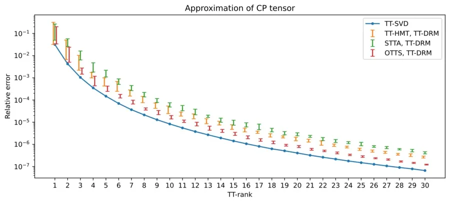
In the plot above we have taken a 10x10x10x10x10 CP tensor and computed TT approximations of different ranks. What we see is that all methods have similar behavior, and are ordered from best to worst approximation as TT-SVD > OTTS > TT-HMT > STTA. This order is something we observe in general across many different experiments, and also in terms of theoretical approximation error. Furthermore, even though these last three methods are all randomized, the variation in approximation error is relatively small, especially for larger ranks. Next, we consider another experiment below:

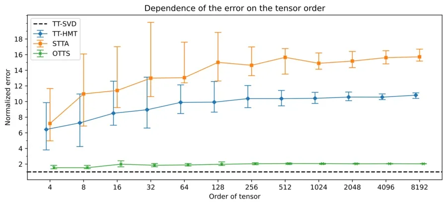
Here we compare the scaling of the error of the different approximation methods as the order of the tensor increases exponentially. The tensor that we’re approximating, in this case, is always a tensor train with a fast decay in its singular values, and the approximation error is always relative to the TT-SVD method. This is because for such a tensor it is possible to compute the TT-SVD approximation in a reasonable time. While all models have similar error scaling, we see that OTTS is closest in performance to TT-SVD. We can thus conclude that all these methods have their merits; we can use STTA if we work with a stream of data, OTTS if we want a good approximation (especially for very big tensors), and TT-HMT if we just want a good approximation and care more about speed than quality.

Conclusion

This sums up, on a high level, what I did in my thesis. There are plenty of things I could still talk about and plenty of details left out, but this blog post is already quite long and technical. If you’re interested to learn more, you’re welcome to read my thesis or send me a message.

My PhD was a long and fun ride, and I’m now looking back on it with nothing but fondness. I enjoyed my time in Geneva, and I’m going to miss some aspects of the PhD life. I have now started a ‘real’ job, and the things I’m working has very little overlap with the contents of my thesis. However, I hope I will be able to discuss some of the cool things I’m working on now, as well as some new personal projects.