Python is generally fast enough – until it’s not. When you reach that point, there are several ways to speed up your Python code. However, one of the most effective approaches is to rewrite the bottleneck in a different language. Traditionally, that language has been C/C++. But now, there’s another contender entering the arena:

That’s right; grab your sunglasses. We’re about to join the cool kids by re-implementing our code in Rust.

The problem

At my workplace, our primary product uses multiple cameras to track people in 3D in real-time. Each camera is designed to detect keypoints—think head, feet, knees, and so on—for each person in view, multiple times per second. These detections are then sent to a centralized application. Since we know the spatial positioning of the cameras, we can triangulate the position of these keypoints by integrating data from multiple cameras.

To grasp how we consolidate information from various cameras, let’s first look at what we can glean from just one camera. If we detect, for instance, a person’s nose in a camera frame (a 2D image), we know the direction in which the nose points from the camera’s perspective—but we can’t determine how far away it is. In geometric terms, we have a line of possible locations for the person’s nose in the 3D world.

We could make an educated guess about the distance based on the average human size, but that’s difficult, error-prone, and imprecise. A more accurate approach is to use multiple cameras. Each camera provides a line of possible locations for a keypoint; thus, by using just two cameras, we can find the intersection of those lines to pinpoint the keypoint’s 3D location.

However, this approach is not foolproof; several sources of uncertainty can compromise the accuracy:

• Cameras might not capture images simultaneously, causing each to deal with a slightly different version of the scene.
• Identifying keypoints is inherently inexact. Could you determine the exact pixel corresponding to someone’s left knee in a photo? Likely not—and neither can machine-learning algorithms. Calibrating the position and orientation of cameras is never perfect; even a minor discrepancy of a centimeter or two can introduce errors.
• Lens distortion is an inevitable aspect of camera technology. While you can correct for it, doing so is never 100% effective.

Adding more cameras could alleviate some of these issues. More lines mean a better intersection point, which can be found by minimizing a (weighted) least squares formula. But if you are like me, then you’re probably just about ready to scream the true solution:

Kalman filters

In our situation, a Kalman filter can essentially be understood in these terms:

• We start with an estimate of both the position and velocity of a keypoint, along with a certain degree of uncertainty.

• As time progresses, this estimate changes—especially if we have an idea of the direction in which the keypoint is moving. However, the uncertainty associated with both the position and velocity will invariably increase. To illustrate, if I see someone moving and then close my eyes, I might guess their location 100 milliseconds later. But if you ask about their location or speed next Tuesday, I’d be clueless.

• Each new observation serves to update our existing knowledge about the keypoint’s position and velocity. Due to the inherent imprecision of all observations, the updated estimates are a blend of our previous estimate and the new observation.

• Formalize these steps and toss in some Gaussians, and you’ve got yourself a Kalman filter! We’re going to dive into the specifics right now, but if you’d rather not get into the math, feel free to skip ahead to the

  </math>
  tag.

<math>

The Kalman filter can be thought of as a two-step process: the prediction step and the update step.

Predict step

To warm up, let’s focus on how to model a single, static keypoint. Imagine we have a position $x\in\mathbb R^3$ along with a $3\times 3$ covariance matrix $P$. These represent the mean and variance of a random variable $X(0)$ at the initial time $t=0$.

As time passes, our estimated position $x$ remains unchanged, but the covariance matrix $P$ should grow. To model this, we can turn to Brownian motion and write $X(t) = X(0) + \eta W(t)$ where $W(t)$ represents a Wiener process (or Brownian motion), and $\eta>0$ is the noise level. The expectaton for this is $\mathbb E(X(t))=X(0)=x$, while the variance evolves according to:

Things get more complicated when we introduce a velocity parameter $v\in \mathbb R^3$. Viewing this from the perspective of a stochastic differential equation (SDE), the original equation was

Adding in the velocity $Y(t)$ this then becomes

We can integrate this by first integrating $Y(t)$ to obtain

Which we then can substitue to get

Finally integrating this we obtain

You’ll notice the last term is not Gaussian. Still, with some standard mathematical tricks (Itô’s Lemma), we find:

In summary, our predict step can be represented as:

While the math wasn’t overly complicated, the intricacy quickly scales with more complex stochastic differential equations. Analytical integration may not always be feasible, making numerical or Monte-Carlo methods an alternative, albeit costly, approach.

Fortunately, if our prediction is linear, we can simplify things considerably. In our case, the function $(x,v)\mapsto (x+vt,v)$ is indeed linear. Let’s denote this map by $F_t$. Now, we encapsulate both $(x_k,v_k)$ together into a single variable $x_k\in\mathbb R^6$, with the covariance $P$ being a $6\times 6$ matrix. Ignoring the $(\eta_vt^3/3)I$ term, the update step simplifies to:

where $Q=\mathrm{diag}(\eta_x,\eta_x,\eta_x,\eta_v,\eta_v,\eta_v)$. We use $\overline{x_{k-1}}$ for the estimate of the state at step $k-1$, acknowledging that we don’t know the actual value. As long as long as our model function $F_t$ is linear, this approximation will suffice. However if $F_t$ is nonlinear, then we’re in trouble, but we’ll see more on that later.

Update step

After the prediction step, we move from an initial state $x_{k-1}$ to an estimated $\hat x_k$. This is an estimate of the true state $x_k$ of the system at time $t_k$, based on our estimate at time $t_{k-1}$. At the same time, we observe the system and obtain a measurement $z_k$ of the system.

Unfortunately the measurement $z_k$ does not live in the same space as the state $x_k$. For example, $z_k$ might represent a 2D observation while $x_k$ represents a position+velocity in 3D.

To go from the ‘model space’ to the ‘measurement space’ we introduce a matrix $H$. In the context of tracking a koving keypoint for instance, this matrix is a $3\times 6$ matrix given blockwise as $(I_3\,\mathbf 0)$ where $\mathbf 0$ is a $3\times 3$ matrixof zeros. This matrix is simply the act of ‘forgetting’ the velocity and only keeping the position.

Our goal is now to derive an estimate $(\overline x_k, P_k)$ for the state $x_k$ at time $t_k$ by incorporating both the previous estimate $\hat x_k$ and the observation $z_k$. In order to do that, we lean on 3 assumptions:

1. The estimate $(\hat x_k,\hat P_k)$ is accurate. That is, we assume $\hat x_k$ is a sample of the distribution $N(x_k,\hat P_k)$.
2. The observation $z_k$ is a direct measurement of $x_k$ with an error $R$, in other words $z_k$ is a sample of $N(Hx_k, R)$
3. There is a matrix $K$, known as the Kalman gain,such that $\overline x_k = \hat x_k+K(z_k-H\hat x_k)$

The last assumption is not really an assumption of the model, but more a convenience to make the math work out. With this assumption we can derive an ‘optimal’ estimate of the true state $x_k$. None of these assumptions are realistic. For instance, in our simple Bayesian analysis of the prediction step we have already noted that the prediction step used by the Kalman filter is an approximation. The second point assumes that the measurement error is exactly Guassian, which is rarely true in practice. Nevertheless, these assumptions make for a good model that can actually be used for practical computations.

Deriving the optimal value of the Kalman gain $K$ is a little tricky, but we can relatively easily use the assumptions above to find a formula for the new error estimate $P_k$. We can define $P_k$ as $\mathrm{cov}(\overline x_k - x_k)$. Then we make several observations:

• By assumption $\mathrm{cov}(x_k - \hat x_k) = \hat P_k$.
• We can write $z_k$ as $Hx_k+v$, where follows a normal distribution $v\sim N(0,R)$ and is independent of the other random variables.

The rest is a straightforward computation using properties of covariance:

Now, let’s tackle the question of how to calculate the optimal value for the Kalman gain. To do this, we first need to clarify what “optimal” signifies in this setting. In this context optimal refers to the value of $K$ that minimizes the expected residual squared error $\mathbb{E}\|\overline x_k-x_k\|^2$. Using some tricks from statistics and matrix calculus it turns out that the opimal Kalman gain takes the following fomr:

where

which is just the covariance matrix of the residual $z_k-H\hat x_k$.

In summary, using several assumptions we can use prior estimate $\hat x_{k}$ and an observation $z_k$ to get an improved estimate $\overline x_k$. This is all a Kalman filter is: we alternate predict and update steps to always have an up-to-date estimate of the models state.

Unscented Kalman filters

To derive the prediction and update steps of the Kalman filter we had to make one ‘stinky’ assumption. It has nothing to do with the approximation we made in the prediction step, or the 3 assumptions I listed in the update step. Rather it’s the assumption that the transition map $F_t$ and the measurement map $H$ are linear maps.

In the case of a moving keypoint both $F_t$ and $H$ were linear. However this is not always the case in more complex systems. Take camera observations as an example. Even ignoring lens distortion, the measurement $H$ is still a projective transformation, not a linear one. To understand why, consider the fact that if we move a point very close to a camera 1cm to the left, it might move many pixels on the image. In contrast,if that same point is several meters away then the same movement will result in a change of 1-2 pixels at best.

So why do we need the linearity assumption? Simply put, if $x$ is Gaussian then so are $F_tx$ and $Hx$, but this is only true for linear maps. One can approximate $F_tx$ and $Hx$ by a Gaussian using a linear approximation of the functions $F_t$ and $H$. However, has its downsides: a) the approximation may be innacurate, and b) computing the linear approximaton requires computing the Jacobian, which may be challenging and computationally expensive.

In summary for a non-linear function $f$ and a gaussian $x\sim N(\mu,\Sigma)$ we need an effective way to estimate the mean $\mathbb E(f(x))$ and covariance $\mathrm{cov}(f(x))$. One method that always works is Monte-Carlo estimation: we simply take lots random of samples $(x_1,\ldots,x_N)$ of $x$, and then compute the mean and covariance of $(f(x_1),\ldots,f(x_N))$. The only issue with this is that we need many samples in order to get an accurate estimate.

Sigma points and the unscented transform

Why rely on random sampling to estimate the mean and covariance of $f(x)$, when we can go with deterministic sampling and pick a robust set of samples $(s_1,\dots,s_N)$. These points are called sigma points. Using these, we can estimate the mean of $f(x)$ through a weighted mean $\mu=\sum_{i=1}^Nf(s_i)W^a_i$. To estimate the covariance we use $\mu$ and a second set of weights to get: $\Sigma = \sum_i W_i^c (f(s_i)-\mu)(f(s_i)-\mu)^\top$. This method is known as the unscented transform (UT). It takes a mean and covariance of a Gaussian $X$ and uses sigma points to estimte the mean and covariance of the transformed variable $f(X)$.

So, how do we pick these sigma points $s_i$ and the associated weights $W^a$ and $W^c$? Technically, any set of points could work, so long as, if $f$ is the identity function, we get the original mean and covariance back. However, most people use a particular algorithm developed by van der Merwe. This algorithm uses three parameters $\alpha, \beta,\kappa$ . Given input mean and covariance $(\mu,\Sigma)$, the algorithm defines:

Here, $n$ is the dimension of $\mu$ and $\lambda := \alpha^2(n+\kappa)-n$. Note the use of the matrix square root which is well-defined for symmetric positive semidefinite matrices – i.e. covariance matrices. You can calculate the matrix square root for example using the singular value decompositon or the Cholesky decomposition. Here are the equations for the weights:

Since these weights don’t depend on $\mu,\Sigma$, we only have to compute them once.

In summary, the unscented transform provides a good estimate of the mean and covariance of $f(X)$ at the cost of:

• $2n+1$ evaluations of the function $f$
• Computing a matrix square root of an $n\times n$ matrix (cost: $O(n^3)$)

In return:

• No need to compute a Jacobian of $f$
• A more accurate estimate if $f$ is non-linear

On top of that, the implementation is not difficult.

Finally you may wonder where the name ‘unscented’ came from. As I alluded to, this is simply because creator, Jeffrey Uhlmann, thought the algorithm was cool and “doesn’t stink”.

Unscented Kalman Filter

Armed with the unscented transform, you only need minor modifications to the Kalman filter algorithm to account for non-linear functions. Let’s first look at the predict step as it used to be:

What happens here is that we have as input a Gaussian $(x,P)$, we then transform it with $F_t$ to get a Gaussian $(F_tx,\, F_tPF_t^\top)$, and then finally we add some extra noise in the shape of $Q$.

Instead of a linear map $F_t$, we now have a non-linear ‘process model’ $f_t$. We just have to swap the estimates of the mean and covariance with those provided by the unscented transform:

Here, $s_i$ are the sigma points derived from $(x_{k-1},P_{k-1})$. While this seems complex, we can rewrite it using the unscented transform $\mathrm{UT}[f_t]$ to get:

That’s not too bad! This also shows you could actually swap out the unscented transform for any method of estimating the mean/covariance of $f_t(X)$.

Then what about the predict step? We have our estimate $(\hat x_k,\hat P_k)$ and an observation $(z_k, R)$. Instead of a measurment matrix $H$, we have a measurment function $h$. We start by applying the unscented transform to the estimate to put it in the measurement space:

Then we calculate the ‘cross-variance’ beween $(\mu_z,\Sigma_z)$ and $(\hat x_k,\hat P_k)$. If $\{s_i\}$ are the sigma points associated to $\mathrm{UT}[h](\hat x_k,\hat P_k)$, then this cross-variacne $P_{xz}$ is defined by:

The cross-variance takes on the role of the matrix $S$ in the original kalman filter. From here we find the Kalman gain as:

Ffinally our new estimate $(x_k,P_k)$ becomes:

And so the unscented kalman filter is born! This concludes the mathematical part of this blog post. Coming up next, we’ll dive into my implemenaton.

</math>

<code>

Let’s put the unscented Kalman filter to work on an actual problem. Not just to see Kalman filters in action, but also to understand why I needed to speed it up.

Model problem

Let’s go back to the beginning of this post. We’re dealing with multiple cameras capturing a person’s movement. A machine learning algorithm is kind enough to give us the ‘keypoints’ on the skeleton of the person (e.g. nose, left elbow, right knee, etc.). Our mision is to turn these 2D pixel positions to 3D coordinates.

To paint a clearer picture, I made a little simulation of a keypoint moving around in 3D projcted down to the viewpoint of two cameras. Below you can see two plots showing what each of the two cameras can see. Thanks to he noise I added the cameras don’t see a smooth curve at all. This is pretty much what you would get when applying machine learning pose detection algorithms on real footage too.

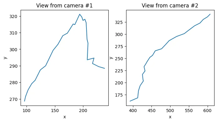
To model this problem we use a model dimension of $6$ (that’s position plus vecocity) and a measurement dimension of 2 (the pixels on a screen).

The measurement function takes in two arguments; the position and an integer indicating the camera number (this is something that we’ll get back to later). To turn this function into an object that Rust can understand, we use the

dim_x = 6
dim_z = 2


@measurement_function(dim_z)
def h_py(x: np.ndarray, cam_id: int) -> np.ndarray:
    pos = x[:3]
    if cam_id == 0:
        return cam1.world_to_screen_single(pos)
    elif cam_id == 1:
        return cam2.world_to_screen_single(pos)
    else:
        return np.zeros(2, dtype=np.float32)


@transition_function
def f_py(x: np.ndarray, dt: float) -> np.ndarray:
    position = x[:3]
    velocity = x[3:]
    return np.concatenate([position + velocity * dt, velocity])

Next we need something to generate sigma points, as well as something to do the heavy lifting of the unscented Kalman filter algorithm. The Kalman filter algorithm needs matrices $Q$, $R$ and $P$ which we’ll need t set as well.

We actually only changed the value of $Q$ from its default, as $P$ and $R$ are fine if they’re an identity matrix in this case. If you have a really good theoretical model, you might be able to derive good values for $Q$, $R$ and $P$. In practice though, you’re just going to have to fiddle around with it until it works.

sigma_points = SigmaPoints.merwe(dim_x, 0.5, 2, -2)
kalman_filter = UKF(dim_x, dim_z, h_py, f_py, sigma_points)


kalman_filter.Q = np.diag([1e-2] * 3 + [3e1] * 3).astype(np.float32)
kalman_filter.R = np.eye(2).astype(np.float32)
kalman_filter.P = np.eye(6).astype(np.float32)

Now we’re going to alternatively do a predict and update step from the point of view of either camera. To tell the Kalman filter which camera is making the observation we use the

predictions_list = []
for p1, p2 in zip(
    proj_points_obs1, proj_points_obs2
):
    kalman_filter.update_measurement_context(0)
    kalman_filter.predict(dt)
    kalman_filter.update(p1)
    predictions_list.append(kalman_filter.x)

    kalman_filter.update_measurement_context(1)
    kalman_filter.predict(dt)
    kalman_filter.update(p2)
    predictions_list.append(kalman_filter.x)

predictions = np.array(predictions_list)  # type: ignore
pos_predictions = predictions[:, :3]

Then finally we are plotting the result below. We see that the Kalman filter is able to track the keypoint quite well in this problem. After taking a bit of time to settle it even gives an accurate estimate of the velocity of the keypoint!

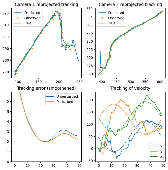
Make it blazingly fast

The implementation above was actually already fully in Rust, and is a lot faster than the Python library

Fortunately it’s not a lot of work to make Rust implementations of these functions and use those instead. To make it more interesting, we will be tracking not just a single keypoint, but 30 keypoints in parallel. This is much closer to the actual use case because a skeleton consists of many keypoints.

Rather than looking at the accuracy, we’re just looking at speed.

Output

Time per keypoint (Rust): 8.1 µs

Output

Time per keypoint (Python}: 120.4 µs
Rust speedup: 14.9x

That’s 15x speedup just for changing out a python functon for a Rust one! Here I used

Originally the idea of

But more importantly, how does this compare to

Output

Time per keypoint (filterpy): 176.4 µs
Rust speedup: 21.8x

We see that

Thoughts on using Rust

This was my first project using Rust and I learned a lot. Not all of my experiences were positive, and I also made some design decisions which I have come to regret. Here are some of my thoughts.

The Measurement function trait

I think Rusts trait system is honestly amazing. All ‘classes’ are just structs which make it extremely clear what all the data is that a ‘class’ uses in its lifetime. Abstract interaction between classes is then done by implementing certain traits.

For example in my code I defined a

One of the reasons we needed this is because measurement functions need context in my usecase. In particular, when we run the update function we need to know for which camera to run this function. There are multiple ways to make this possible, but since I wanted to avoid restrictions on what this context could be, it became a bit of a headache dealing with this.

When using a Kalman filter it is normal to have different sensors (such as different cameras), which means having a different measurement function for each sensor. If the number of sensors is finite, then we don’t actually need an arbitrary object as context. We just need to keep a list of all the measurement functions, and then the only context we need is a single index. Had I made this design decision, my code would likely have been much simpler.

PyO3

C/C++ with a together with a library like pybind is still the go-to for speedin up your Python code. With the PyO3 crate, Rust offers itself as a solid alternative. Defining classes and methods, calling Python code, handling errors, and dealing with the GIL is relatively easy. I think what makes this possible is Rust’s first-class macro system. Still, you do end up with a fair bit of boilerplate. For instance, you need to define getters and setters for every single attribute that you want to expose to Python. As an example, I ended up with 143 lines of code that looks like this in the unscented Kalman filter class alone:

#[getter]
#[pyo3(name = "x")]
pub fn py_get_x(&self, py: Python<'_>) -> PyResult<Py<PyArray1<Float>>> {
    let array = self.x.clone().into_pyarray(py).to_owned();
    Ok(array)
}

#[setter]
#[pyo3(name = "x")]
pub fn py_set_x(&mut self, x: PyReadonlyArray1<Float>) -> PyResult<()> {
    self.x = x.as_array().to_owned();
    Ok(())
}

I understand why it’s necessary, but that doesn’t make it fun.

Furthermore, Rust has good support for generic types. There were quite a few places where defining a struct or trait with generic types would have made my life easier, but this is not supported by PyO3 (at least for now).

As the ecosystem matures a little, I have no doubt things are going to improve even further. But for now, while it isn’t difficult per se, it still can be a bit tedious to write Python modules in Rust.

ndarray vs numpy

One reason why I really enjoy writing numerical code in Python is because of numpy and its surrounding ecosystem. Rust is faster, but without good libraries for numerical array programming, it would not be so useful for me. The main library in this area is the

For instance, in Python we might write

Profiling

Whenever writing code were speed matters, profiling is your best friend. In this particular project I was using

Conclusion

Rust is a pretty compelling tool for writing fast code as part of a larger Python code base. I like the language, and I am eager to use more of it. I don’t know if the unscented Kalman filter implementation I made will actually end up getting used at my workplace, but it was a nice learning experience regardless. It was also very interesting to actually dive deeper into how (unscented) Kalman filters work, rather than just using them as a tool.

I hope you learned something about Kalman filters, and I’m eager to know how you will use Rust to speed up some of your Python codebse!