Blind Deconvolution #2: Image Priors
Published on 9th of April, 2021.
This is part two in a series on blind deconvolution of images. In the previous part we looked at non-blind deconvolution, where we have an image and we know exactly how it was distorted. While this situation may seem unrealistic, it does occur in cases where we have excellent understanding of how the camera takes images; for example for telescopes or microscopes which always work in the same environment.
The next step is then to try to do deconvolution if we have partial information about how the image was distorted. For example, we know that a lens is out of focus, but we don’t know exactly by how much. In that case we have only one variable to control, a scalar amount of blur (or perhaps two if the amount of blur is different in different directions). In this case we can simply try deconvolution for a few values, and look which image seems most natural.
Below we have the image of the St. Vitus church in my hometown distorted with gaussian blur with , and then deblurred with several different values of . Looking at these images we can see that and looks best, and is over-sharpened. The real challenge lies in finding some concrete metric to automatically decide which of these looks most natural. This is especially hard since even to the human eye this is not clear. The fact that looks very good probably means that the original image wasn’t completely sharp itself, and we don’t have a good ground truth of what it means for an image to be perfectly sharp.
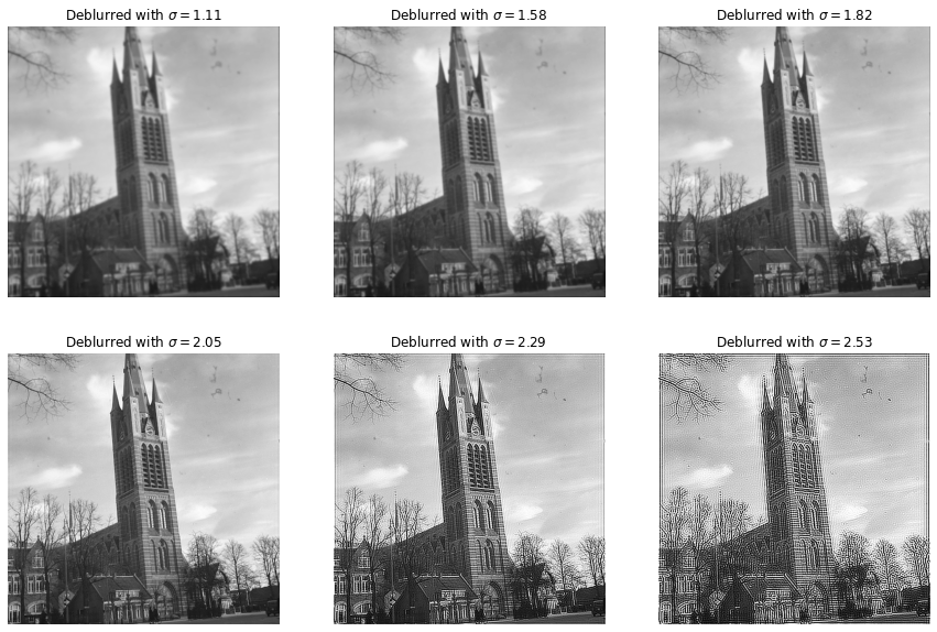
Image priors
Measures of naturality of an image are often called image priors. They can be used to define a prior distribution on the space of all images, giving higher probability to images that are natural over those that are unnatural. Often image priors are based on heuristics, and different applications need different priors.
Many simple but effective image priors rely on the observation that most images have a sparse gradient distribution. An edge in an image is a sharp transition. The gradient of an image measures how fast the image is changing at every point, so a an edge is region in the image where the gradient is large. The gradient of an image can be computed by convolution with different kernels. One such kernel is the Sobel kernel:
Here convolution with gives the gradient in the horizontal direction, and it is large when encountering a vertical edge, since the image is then making a fast transition in the horizontal direction. Similarly gives the gradient in the vertical direction. If is our image of interest, we can then define the gradient transformation of by
Below we can see this gradient transformation in action on the six images shown above:
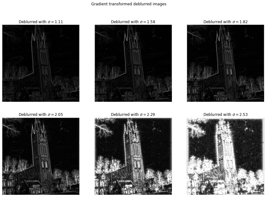
Here we can see that the gradients become larger in magnitude as increases. For we see that a large part of the image is detected as gradient – edges stopped being sparse at this point. For the first four images we see that the edges are sparse, with most of the image consisting of slow transitions.
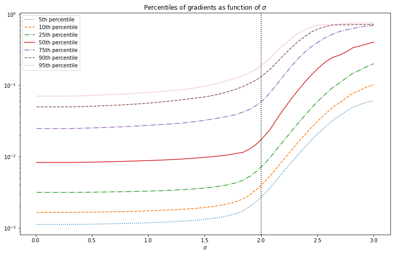
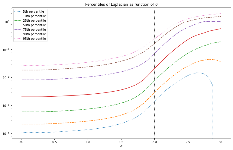
Below we look at the distribution of the gradients after deconvolution with different values of . We see that the distribution stays mostly the constant, slowly increasing in overall magnitude. But near , the overall magnitude of gradients suddenly increases sharply.
This suggests that to find the optimal value of we can look at these curves and pick the value of where the gradient magnitude starts to increase quickly. This is however not very precise, and ideally we have some function which has a minimum near the optimal value of . Furthermore this curve will look slightly different for different images. This is a good starting point for an image prior, but is not useful yet.
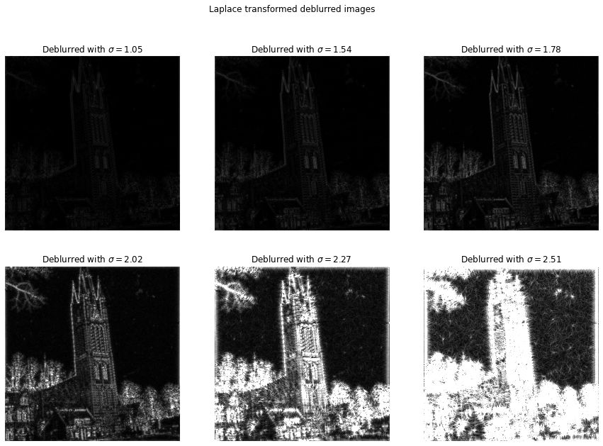
Instead of using the gradient to obtain the edges in the image, we can use the Laplacian. The gradient is the first derivative of the image, whereas the Laplacian is given by the sum of second partial derivatives of the image. Near an edge we don’t just expect the gradient to be big, but we also expect the gradient to change fast. This is because edges are usually transient, and not extended throughout space.
We can compute the Laplacian by convolving with the following kernel:
Note that the Laplacian can take on both negative and positive values, unlike the absolute gradient transform we used before. Below we show the absolute value of the Laplacian transformed images. This looks similar to the absolute gradient, except that the increase in intensity with increasing is more pronounced.
metric
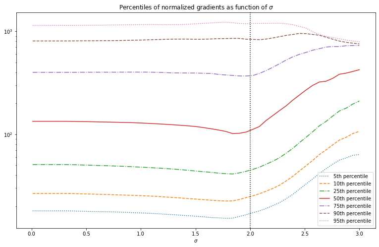
Above we can see that there is an overall increase in the magnitude of the gradients and Laplacian as increases. We want to measure how sparse these gradient distributions are, and this has more to do with the shape of the distribution rather than the overall magnitude. To better see how the shape changes it therefore makes sense to normalize so that the total magnitude stays the same. We therefore don’t consider the distribution of the gradient , but rather of the normalized gradient . Since the mean absolute value is essentially the -norm, this is also referred to as the -norm of the gradients .
The normalized gradient distribution is plotted below as function of , the distributions of the Laplacian look similar. This distribution already looks a lot more promising since the median has a minimum near the optimal value for . This minimum is a passable estimate of the optimal value of for this particular image. For other images it is however not as good. Moreover the function only changes slowly around the minimum value, so it is hard to find in an optimization routine. We therefore need to come up with something better.
Non-local similarity based priors
The prior is a good starting point, but we can do better with a more complex prior based on non-local self-similarity. The idea is to divide the image up in many small patches of pixels with for example . Then for each patch we can check how many other patches in the image look similar to it. This concept is called non-local self-similarity, since it’s non-local (we compare a patch with patches throughout the entire image, not just in a neighborhood) and uses self-similarity (we look at how similar some parts of the image are to other parts of the same image; we never use an external database of images for example).
The full idea is a bit more complicated. Let’s denote each patch by
We consider this patch as a length- vector. Moreover since we’re mostly interested in the patterns represented by the patch, and not by the overall brightness, we normalize all the patch vectors to have norm 1. We then find the closest matching patches, minimizing the Euclidean distance:
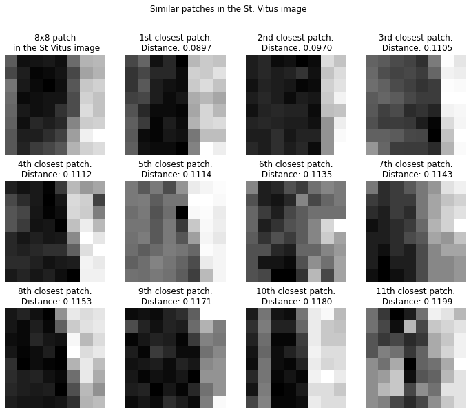
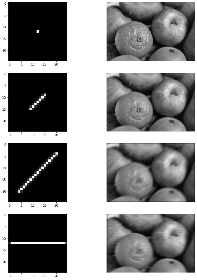
Below we show an 8x8 patch in the St. Vitus image (top left) together with its 11 closest neighbors.
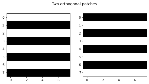
Note that we look at patches closest in Euclidean distance, this does not necessarily mean the patches are visually similar. Visually very similar patches can have large euclidean distance, for example the two patches below are orthogonal (and hence have maximal Euclidean distance), despite being visually similar. One could come up with better measures for visual similarity than Euclidean distance, probably something that is invariant under small shifts, rotations and mirroring, but this would come at an obvious cost of increased (computational) complexity.
The closest patches together with the original patch are put into a matrix, called the non-local self-similar (NLSS) matrix . We are interested in some linear-algebraic properties of this matrix. One observation is that the NLSS matrices tend to be of low rank for most patches. This essentially means that most patches tend to have other patches that look very similar to it. If all patches in are the same then its rank is 1, whereas if all the patches are different then is of maximal rank.
However, taking the rank itself is not necessarily a good measure, since it is not numerically stable. Any slight perturbation will always make the matrix of full rank. We rather work with a differentiable approximation of the rank. This approximation is based on the spectrum (singular values) of the matrix. In this case, we can consider the nuclear norm of . It is defined as the sum of the singular values:
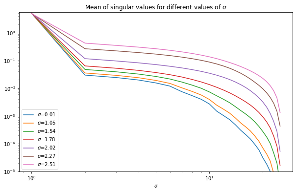
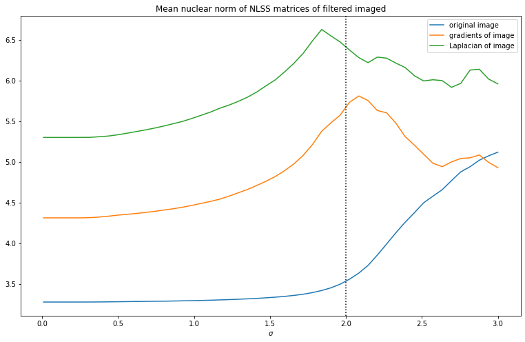
where is the th singular value. Below we show how the average singular values change with scale of the deconvolution kernel for the NLSS matrices for 8x8 patches with 63 neighbors (so that the NLSS matrix is square). We see that in all cases most of the energy is in the first singular value, followed by a fairly slow decay. As increases, the decay of singular values slows down. This means that the more blurry the image, the lower the effective rank of the NLSS matrices. As such, the nuclear norm of the NLSS matrix gives a measure of the amount of information in the picture.
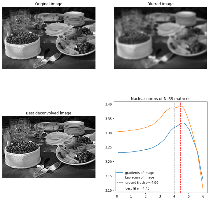
We see that the spectrum of the NLSS matrices seem to give a measure of ‘amount of information’ or sparsity. Since we know that sparsity of the edges in an image gives a useful image prior, let’s compute the nuclear norm of each NLSS matrix of the gradients of the image. We can actually plot these nuclear norms as an image. Below we show this plot of nuclear norms of the NLSS matrices. We can see that the mean nuclear norm is biggest at around the ground truth value of .
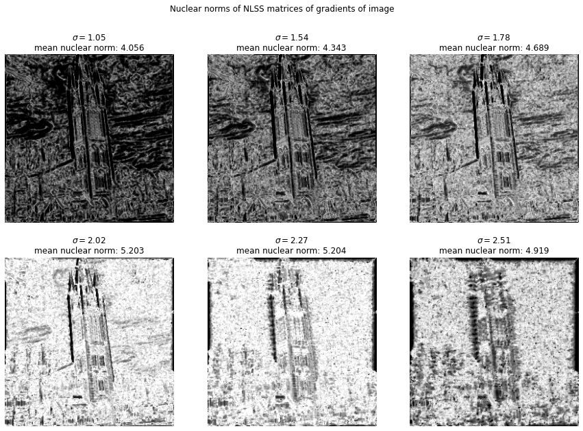
It is not immediately clear how to interpret the darker and lighter regions of these plots. Long straight edges seem to have smaller norms since there are many patches that look similar. Since the patches are normalized before being compared, the background tends to look a lot like random noise and hence has relatively high nuclear norm. However, we can’t skip this normalization step either, since then we mostly observe a strict increase in nuclear norms with .
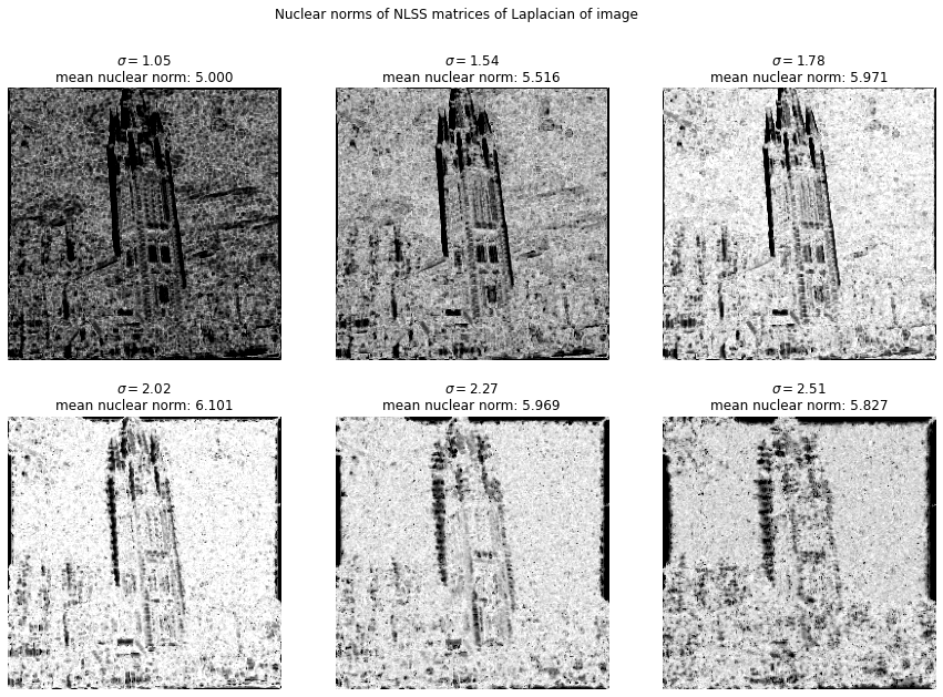
Repeating the same for the Laplacian gives a similar result:
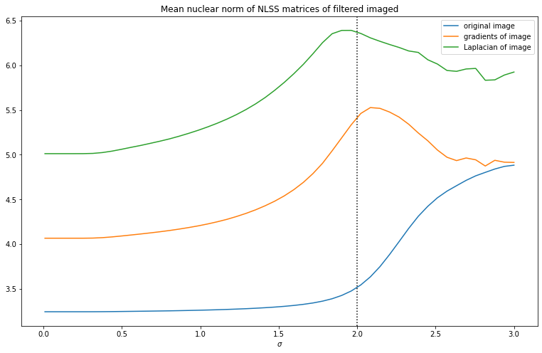
Now finally to turn this into a useful image prior, we can plot how the mean nuclear norm changes with varying . Both for the gradients and Laplacian of the image we see a clear maximum near , so this looks like a useful image prior.
There are a few hyperparameters to tinker with for this image prior. There is the size of the patches taken, in practice something like 4x4 to 8x8 seems to work well for the size of images we’re dealing with. we can also lower or increase the number of neighbors computed. Finally we don’t need to divide the images into patches exactly. We can oversample, and put a space of less than pixels between consecutive patches. This results in a less noisy curve of NLSS nuclear norms, at extra computational cost. We can on the other hand also undersample and only use a quarter of the patches, which can greatly improve speed.
The image above was made for patches with 36 neighbors. Below we make the same plot with patches, but only taking 1/16th of the patches and only 5 neighbors. This results in a much more noisy image, but it runs over 10x faster and still gives a useful approximation.
One final thing of note is how the NLSS matrices are computed. Finding the closest patches through brute-force methods of computing the distance between each pair of patches is extremely inefficient. Fortunately there are more efficient ways to solving this similarity search problem. These methods usually first make an index or tree structure saving some information about all the data points. This can be used to quickly find a set of points that are close to the point of interest, and searching only within this set significantly reduces the amount of work. This is especially true if we only care about approximately finding the closest points, since this mean we can reduce our search space even further.
We used Faiss to solve the similarity search problem, since it is fast and runs on GPU. There are many packages that do the same, some faster than others depending on the problem. There is also an implementation in
At the end of the day the bottleneck in the computation speed is the computation of the nuclear norm. This in turn requires computing the singular values of tens of thousands of small matrices. Unfortunately CUDA only supports batched SVD computation of matrices of at most 32x32 in size, and indeed if we use 5x5 patches or smaller, we can make this up to 4x faster by doing the computation on GPU on my machine.
Testing the image prior
The nuclear norms of NLSS matrices seem to give a useful image prior, but to know for sure we need to test it for different images, and also for different types of kernels.
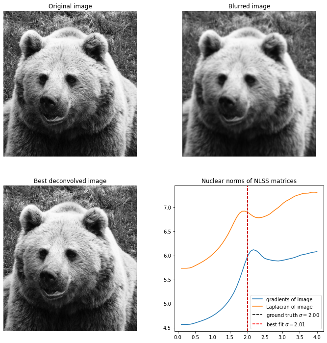
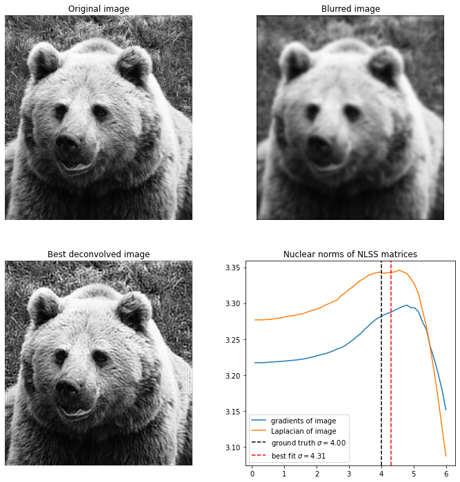
To estimate the best deconvolved image, will take the average of the optimal value for the NLSS nuclear norms of the gradient and Laplacian. This is because it seems that the Laplacian usually underestimates the ground truth value whereas the gradient usually overestimates it. Furthermore, instead of taking the global maximum as optimal value, we take the first maximum. When we oversharpen the image a lot, the strange artifacts we get can actually result in a large NLSS nuclear norm. It can be a bit tricky to detect a local maximum, and if the initial blur is too much then the prior seems not to work very well.
First let’s try to do semi-blind deconvolution for Gaussian kernels. That is, we know that the image was blurred with a Gaussian kernel, but we don’t know with what parameters. We do this for a smaller and a larger value for the standard deviation , and notice that for smaller the recovery is excellent, but once becomes too large the recovery fails.
All the images we use are from the COCO 2017 dataset.
First up is an image of a bear, blurred with Gaussian kernel. Deblurring this is easy, and not very sensitive on the hyper parameters used.
Here is the same image of the bear, but now blurred with , and it becomes much harder to recover the image. I found that the only way to do it is to reduce the patch size all the way to , for higher patch sizes the image can’t be accurately recovered and it always overestimates the value of .
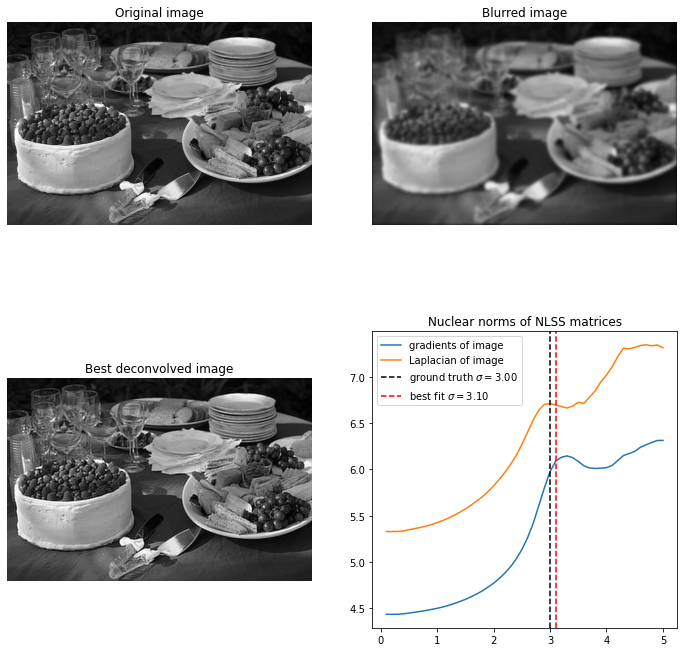
Below is a picture of some food. For recovery is excellent, and again not strongly dependent on hyperparameters. For the problem becomes significantly harder, and it again takes a small patch size for reasonable results.
Now let’s change the blur kernel to an idealized motion blur kernel. Here the point spread function is a line segment of some specified length and thickness, as shown below:
The way I construct these point spread functions is by rasterizing an image of a line segment. I’m sure there’s a better way to do this, but it seems to work fine. The parameters of the kernel are the angle, the length of the line segment and the size of the kernel.
Let’s try to apply the method on a picture of some cows below:
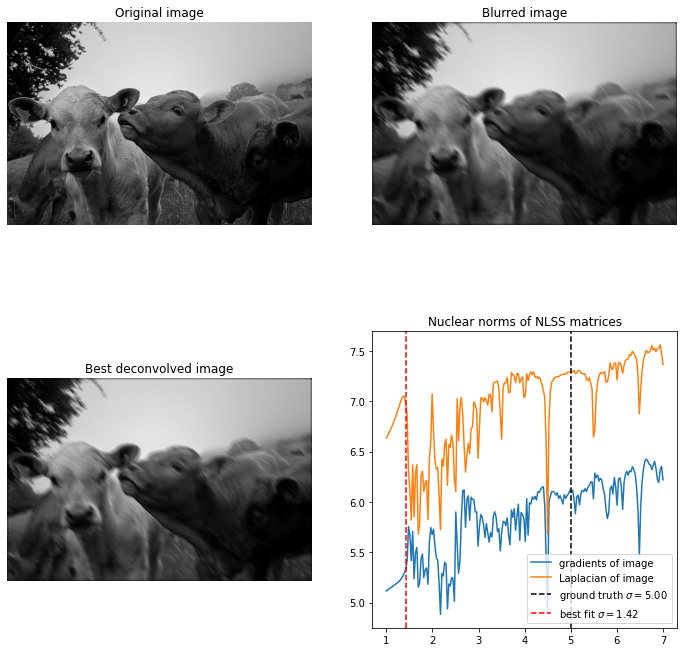
Unfortunately our current method doesn’t work well with this kind of point spread function. The nuclear norm of the NLSS matrices is very noisy. I first thought this could be because the PSF doesn’t change continuously with the length of the line segment. But I ruled this out by hard-coding a diagonal line segment in such a way that it changes continuously, and it looks just as bad.
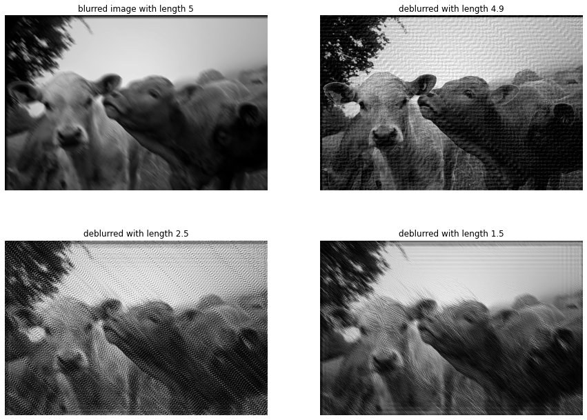
Instead it seems that the (non-blind) deconvolution method itself doesn’t work well for this kernel. Below we see the image blurred with a length 5 diagonal motion blur, and then deconvolved with different values. With the Gaussian blur we only saw significant deconvolution artifacts if we try to oversharpen an image. Here we see very significant artifacts even if the length parameter is less than 5. I think this is because the point spread function is very discontinuous, and hence its Fourier transform is very irregular.
Additionally, the effect of motion blur on edges is different than that of Gaussian blur. If the edge is parallel to the motion blur, it is not affected or even enhanced. On the other hand, if an edge is orthogonal to the direction of motion blur, the edge is destroyed quickly. This may mean that the sparse gradient prior is not as effective as for Gaussian blur. We have no good way to check this however before improving the deconvolution method.
Conclusion
Having a good image prior is vital for blind deconvolution. Making a good image prior is however quite difficult. Most image priors are based on the idea that natural images have sparsely distributed gradients. We observed that the simple and easy-to-compute prior does a decent job, but isn’t quite good enough. The more complex NLSS nuclear norm prior does a much better job. Using this prior we can do partially blind deconvolution, sharpening an image blurred with Gaussian blur.
However, another vital ingredient for blind deconvolution is good non-blind deconvolution. The current non-blind deconvolution method we introduced in the last part doesn’t work well for non-continuos or sparse point spread functions. There are also problems with artifacts at the boundaries of the image (which I have hidden for now by essentially cheating). This means that if we want to do good blind deconvolution, we first need to revisit non-blind deconvolution and improve our methods.
Other posts you may like
Rik Voorhaar © 2024